4D World (X): Rotational Dynamics

/// Note: Although this article extensively discusses fictional physical laws in a fictional four-dimensional world, it also discusses the uniform random distribution laws of unit four-dimensional bivectors from a purely mathematical perspective.

Content Overview

• 4D Dzhanibekov effect
• Multi-body rotating systems with energy exchange
• Random distribution laws of angular momentum
• Principal axis theorem for four-dimensional rigid bodies

The Dzhanibekov Effect

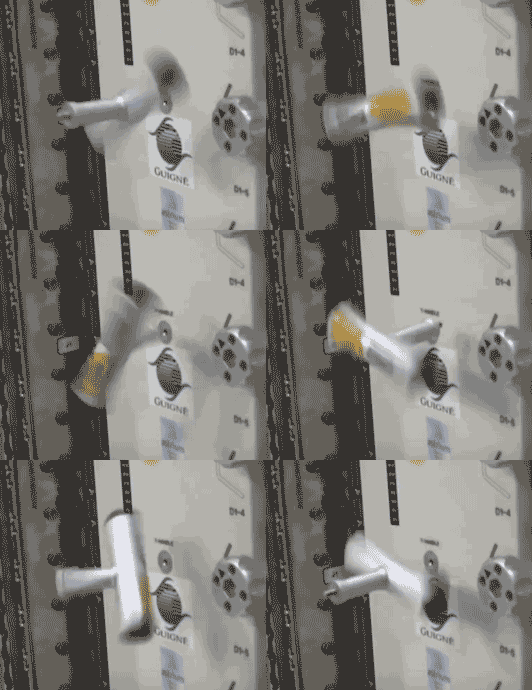
A Soviet cosmonaut was playing with a T-shaped part in space when he accidentally discovered that when the part was made to float and spin rapidly, its rotation direction would suddenly flip from time to time. This phenomenon was later named the Dzhanibekov Effect after him (Джанибеков).

There are many ways to explain this phenomenon, with its root cause stemming from angular momentum conservation and the anisotropy of the handle’s moment of inertia. Let’s start with Newton’s first law, which states that an object not subjected to external forces will maintain uniform linear motion or remain stationary. However, this doesn’t consider the object’s rotation. Should an object not subjected to external forces maintain uniform angular velocity rotation? Not necessarily. Actually, when an object is not subjected to external forces, it’s not the velocity and angular velocity that remain constant, but the momentum and angular momentum. Since momentum equals mass times velocity, and an object’s mass generally doesn’t change, we can deduce that the object’s velocity also happens to remain constant. However, the relationship between an object’s angular momentum and angular velocity is more complex. Take a tennis racket for example - due to its different dimensions in various directions, the difficulty of rotation around different axes varies, meaning each direction has a different moment of inertia. Angular momentum equals moment of inertia times angular velocity. When the object rotates, these axes also rotate with it, and the moment of inertia in each direction changes. To maintain constant total angular momentum output, the angular velocity must change with the rotation axis to offset the changes in moment of inertia. This is why a part rotates and flips by itself when not subjected to external forces. If the rotating object has uniform symmetry, like a cube or sphere, with the same moment of inertia in all directions, it will only rotate uniformly without the Dzhanibekov effect.

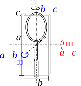
Actually, the conditions for this effect are quite stringent. It also requires that the object’s initial rotation axis be the intermediate axis between the long and short axes. What does this mean? From three-dimensional rigid body mechanics analysis, we know that any rigid body’s moment of inertia is equivalent to that of a triaxial ellipsoid or cuboid - describing the moments of inertia of the three principal axes is sufficient to determine the entire object’s rotational behavior. Therefore, we can treat the tennis racket as equivalent to a rectangular plate. The figure above shows the tennis racket’s rotation around the long axis $a$, short axis $c$, and intermediate axis $b$. Only rotation around the intermediate axis (marked in red in the figure) is unstable and produces the Dzhanibekov effect. This theorem about rotational stability is also known as the tennis racket theorem. There are mechanics-based explanations, energy-based explanations, and explanations based on stability analysis of Euler’s rotation differential equations for why only the intermediate axis rotation is unstable, but this isn’t the focus of this article, so I won’t elaborate further.

Four-Dimensional Case

Although we cannot actually conduct experiments in an imagined four-dimensional space to witness four-dimensional effects, we can simulate them through the physics engine in Tesserxel. The specific physics formulas used in the engine are provided in the appendix. First, to achieve rotational instability, we must find an object with four unequal “axes” - the simplest being a hyperrectangular box. Unlike in three dimensions, rotation in four-dimensional space occurs in planes, and pairwise combinations of principal axes yield six directions, with six possible initial rotation positions.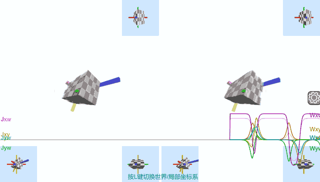

Let the hyperrectangular box have 4 unequal edges $a$, $b$, $c$, $d$, where $a < b < c < d$. Through numerical simulation, I discovered the following patterns:

1. Initial rotation planes chosen as $ab$, $bc$, or $cd$ are all stable. $ab$ is similar to the three-dimensional longest axis with the smallest moment of inertia; $cd$ is similar to the three-dimensional shortest axis with the largest moment of inertia; although the rotation plane $bc$ is a type of “intermediate axis,” it is stable. Click here to simulate $bc$ plane rotation online in Tesserxel.
2. When the initial rotation plane is chosen as $ac$ or $bd$, intermediate axis instability similar to the three-dimensional case occurs, producing a Dzhanibekov effect almost identical to the three-dimensional situation. Click here to simulate $ac$ plane rotation online in Tesserxel.
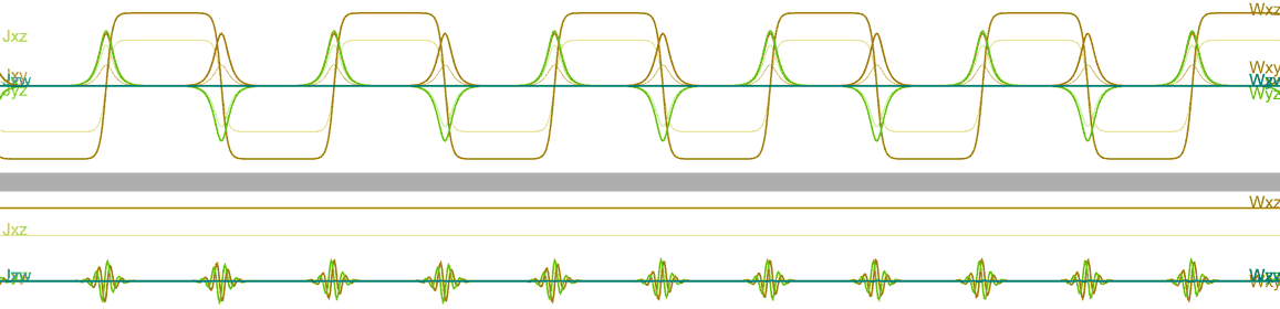
3. When the initial rotation plane is chosen as $ad$, the rotation is also unstable, with two different periods of reverse rotation alternating - a phenomenon unique to the four-dimensional Dzhanibekov effect. Since each period causes the rotation direction to flip, the combined action of two different periods makes the angular momentum change curve in the rigid body’s local coordinate system look like a pulse width modulation (PWM) waveform. Click here to simulate $ad$ plane rotation online in Tesserxel.

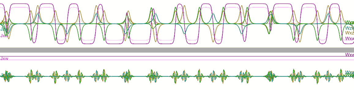
In the above online simulations, you can press the L key on the keyboard to switch between the inertial coordinate system and the rigid body’s local coordinate system. The rigid body’s axes from smallest to largest correspond to coordinates $x$, $y$, $z$, $w$ respectively. We can observe:

1. In the inertial coordinate system: In any case, all components of the object’s angular momentum (represented by letter J) remain constant as straight lines, representing absolute conservation of angular momentum. In scenarios with the Dzhanibekov effect, we can see that besides the component corresponding to the initial angular velocity barely changing, some smaller components of other angular velocities (represented by letter W) temporarily appear when the rotation direction reverses.
2. After switching to the local coordinate system, we can see that the direction of the component corresponding to the initial angular velocity also flips each time the object reverses.

Why do the angular velocity behaviors in these two coordinate systems differ so drastically? It’s said that when cosmonaut Dzhanibekov accidentally discovered this effect in space, he was very worried that Earth’s rotation might suddenly flip over one day. Of course, we later learned that Earth’s rotation axis is in the shortest direction of a triaxial ellipsoid, making the rotation stable, so there’s no need to worry about such things happening. Let’s suppose Earth’s rotation axis is the intermediate axis - originally Earth rotates from west to east, with the sun rising in the east and setting in the west. After Earth’s north and south poles flip, since the total angular momentum direction doesn’t change, from the universe’s inertial frame Earth still rotates from west to east. However, people on Earth would feel differently: the original east-west-south-north directions have become the actual west-east-north-south directions due to Earth’s flip. People on the ground would feel the sun rises in the west and sets in the east, but people in space still think the sun rises in the east and sets in the west. Hopefully readers can now understand why angular velocity in the inertial frame barely changes while it periodically reverses in the local frame.

Summary of Stability Rules

Observing the three cases above, it’s not hard to find the following patterns for stability judgment: If the plane is spanned by adjacent edges arranged in size order, the rotation is stable; if there’s one edge in between, it produces a single-period Dzhanibekov effect; if there are two edges in between, it produces a double-period Dzhanibekov effect. Additionally, I discovered some rules about isoclinic rotation:

1. If the initial rotation is an isoclinic double rotation, the rotation is stable, such as rotating the $ac$ and $bd$ planes at the same angular velocity: Click here to simulate online in Tesserxel.
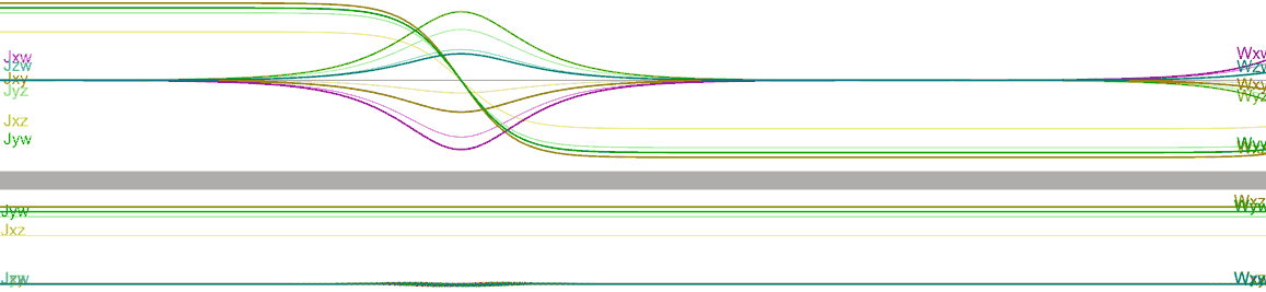
2. For non-isoclinic double rotation, whichever of the two absolutely perpendicular rotations has greater angular velocity will have a more pronounced effect, and the closer the initial rotation is to perfect isoclinic double rotation, the longer the flip period. In the following online simulation, the speed ratio of the two absolutely perpendicular rotations in the double rotation is $15/16$, already quite close to isoclinic, so the direction flip period is particularly long - you need to wait over half a minute to see the angular momentum flip: Click here to simulate online in Tesserxel.

A Brief Aside

The first time I heard about the Dzhanibekov effect was actually when Marc ten Bosch mentioned the four-dimensional Dzhanibekov effect in his paper “𝑁-Dimensional Rigid Body Dynamics”. Then I searched for the three-dimensional case and learned about the Soviet cosmonaut’s story. I then discovered that my four-dimensional engine hadn’t considered the rigid body precession terms caused by non-uniform moments of inertia - I hastily patched this major bug in the engine.

The conclusions in Marc ten Bosch’s paper differ from those in this article. His simulation results indicate that hyperrectangular boxes with four unequal axes will eventually tend toward double rotation as a stable state. However, I believe this result is incorrect: Imagine a hyperrectangular box that’s fairly close to a hypercube - its moments of inertia in various directions differ but not significantly. If the initial rotation is a simple rotation with corresponding angular velocity as a simple bivector, although the total angular momentum might not be a simple bivector, it shouldn’t deviate too much. If it evolves to isoclinic double rotation, the angular velocity would be a self-dual or anti-self-dual bivector, too different from a simple bivector to satisfy conservation of total angular momentum. Marc himself noted that numerical errors accumulated in his implicit solver causing angular velocity to decrease noticeably (Tesserxel uses the highly accurate fourth-order Runge-Kutta method). Since I don’t know how he calculated it, I can only guess that the same reason likely caused the erroneous convergence to isoclinic rotation results. My solutions in both Mathematica and my own TypeScript-written Tesserxel physics engine indicate that four-dimensional freely rotating rigid bodies do not spontaneously tend toward stable isoclinic double rotation states.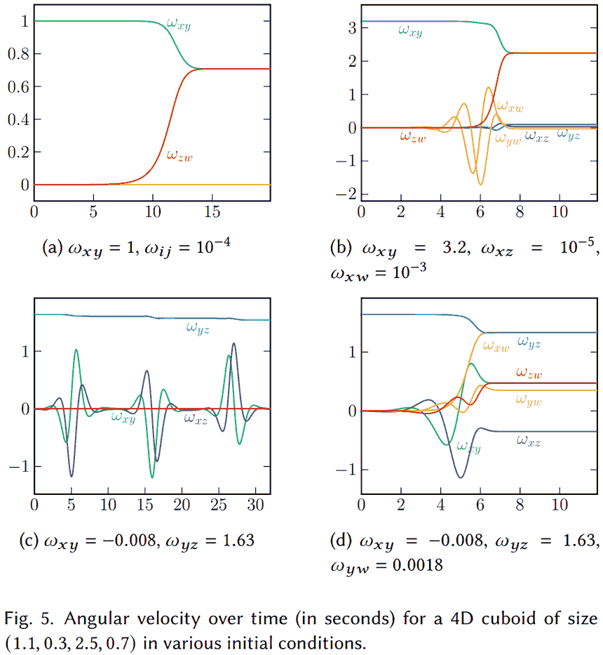

Multi-Body Rotating Systems with Energy Exchange

What we just saw was the free rotation of an isolated rigid body. If there are losses inside the rigid body, such as a cup filled with liquid, Wikipedia says it will gradually tend toward the lowest energy stable state while maintaining constant total angular momentum. This raises an interesting question: What is the most likely rotation pattern for a general four-dimensional planet? Is simple rotation more likely, or is isoclinic double rotation or general double rotation more likely? Someone on the Higher Space forum believes that planets with isoclinic double rotation have the same velocity magnitude at all points, representing an energy-equipartitioned stable state. In simple rotation, the equator has the highest velocity while the poles have zero velocity, which is not an equilibrium state, so eventually all planets will evolve to isoclinic double rotation. However, like Marc ten Bosch’s oversight, an isolated planet cannot directly evolve from simple rotation to isoclinic rotation under the constraint of total angular momentum. The only opportunity is during the early evolution of the planetary system in which the planet forms. Since four-dimensional celestial mechanics has many fundamental bugs - orbital systems are unstable in gravitational fields with inverse cube decay - we won’t discuss here how specific planets acquire initial angular momentum. Instead, let’s look at a thermodynamic “toy model”: Imagine an absolutely smooth hyperspherical cavity filled with a bunch of small balls (actually hyperspheres) with randomly distributed initial velocities. They freely collide inside like air molecules doing Brownian motion. The ball surfaces have friction allowing them to exchange momentum and angular momentum, but they can’t obtain additional angular momentum from the hypersphere walls, thus maintaining conservation of total angular momentum. After reaching equilibrium after some time, what is the distribution pattern of these small balls’ angular velocities? I placed 40 small balls in Tesserxel and marked each ball’s degree of isoclinicity in angular velocity - self-dual as 1, simple as 0, anti-self-dual as -1. The specific calculation formula is here. Click here to simulate online in Tesserxel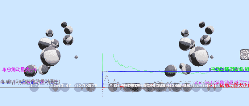

Since they collide within the hyperspherical shell and the shell cannot provide angular momentum, the total angular momentum remains conserved. However, unlike a single isolated rigid body, the system’s angular momentum consists of two parts: orbital angular momentum and spin angular momentum. These two parts are individually non-conserved; only their sum is conserved. Here’s a simple example to deepen understanding: Imagine two astronauts of nearly equal mass in vacuum, very close to each other, maintaining relative rest. They extend their hands and high-five in the manner shown by the green arrows in the figure below. The interaction force causes them to start rotating and move apart. It’s easy to see that they both rotate in the same direction, seemingly violating conservation of total angular momentum. Actually, besides spin having angular momentum, their center of mass motion also has orbital angular momentum, and its direction is clockwise, opposite to the counterclockwise spin direction, so total angular momentum is still conserved.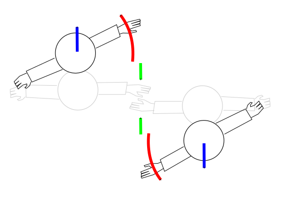
Through Tesserxel simulation, I found that these small balls do sometimes collectively tend toward isoclinic double rotation. If the initial spin angular momentum has a larger self-dual component, they’ll eventually all tend toward self-dual angular momentum. If the initial rotation has a larger anti-self-dual component, they’ll eventually all tend toward anti-self-dual angular momentum.


If the initial angular momentum is simple, the final steady state could be either self-dual or anti-self-dual, sometimes showing completely uniform random distribution with no visible convergence trend - simulation time might be too short and subsequent convergence to dual states can’t be ruled out. I also accidentally discovered one case of simultaneous convergence toward both ends, but this situation was hardly reproduced afterward.

Although I can’t guarantee these patterns aren’t artifacts caused by computational errors, these phenomena are at least consistent with conservation of total angular momentum, because the extra isoclinic components in spin can be offset by opposite extra components in orbital angular momentum. In this sense, it makes sense for planetary evolution to tend toward isoclinic double rotation. However, the stability of four-dimensional celestial orbits doesn’t allow us enough time for planets to fully collide and exchange angular momentum, so it’s hard to say actual planets are all in isoclinic double rotation. Since we can’t imagine a reasonable planetary system evolution process to derive planetary angular momentum, if we directly assume planets have randomly directed angular momentum, how should simple and compound bivectors be distributed to be truly random? Below we assume angular momentum has magnitude 1 and explore how to uniformly generate randomly directed angular velocity bivectors.

Random Distribution Laws of Angular Momentum

How do we randomly generate an arbitrary unit bivector? Here are several methods I’ve thought of:

1. Here I’ve already introduced an algorithm for generating random simple unit bivectors based on left-right isoclinic decomposition, but it can’t generate compound bivectors. There’s reason to believe that superimposing enough of these random bivectors can approximate arbitrary uniformly distributed random bivectors. This is actually equivalent to a random walk model in three-dimensional space: Each time we add a random simple bivector, it’s equivalent to taking equal-distance random walks in both the three-dimensional self-dual and anti-self-dual spaces. The duality of the compound bivector depends on the ratio of random walk distances in the two spaces.
2. Here I’ve already introduced an algorithm based on dual decomposition that can generate random rotations in four-dimensional space. Taking the logarithm of random rotations gives the generator bivector similar to angular momentum, which can be normalized to get randomly distributed bivectors.
3. There’s also a direct brute force approach: Bivectors are just vectors with six degrees of freedom. Generating unit bivectors is actually generating uniformly distributed points on a five-dimensional hypersphere in six-dimensional space.

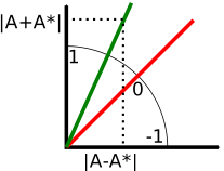
Do these three methods generate bivectors with the same distribution patterns? Obviously these methods are all isotropic in four-dimensional space, so differences are reflected in the distribution of bivector duality - the distribution ratio of self-dual and anti-self-dual components. I specifically defined a duality measure to quantitatively describe it: self-dual has duality 1, anti-self-dual has -1, simple has 0.

Optional Reading: Definition of the Duality Function

Since self-dual and anti-self-dual bivectors have zero for their other component, directly defining ratios would introduce infinity problems, so I converted the ratio through the arctangent function into an angle and normalized it. Let $A$ be a unit bivector, then its duality is defined as

$$\mathrm{duality}(A)={4 \over\pi}(\arctan(|A+A^*|,|A-A^*|)-{\pi\over 4})$$
Its geometric meaning maps the ratio of $x$, $y$ coordinates of points on the unit circle to the ratio of self-dual and anti-self-dual components, using arc length parameters to measure which state it’s closer to.

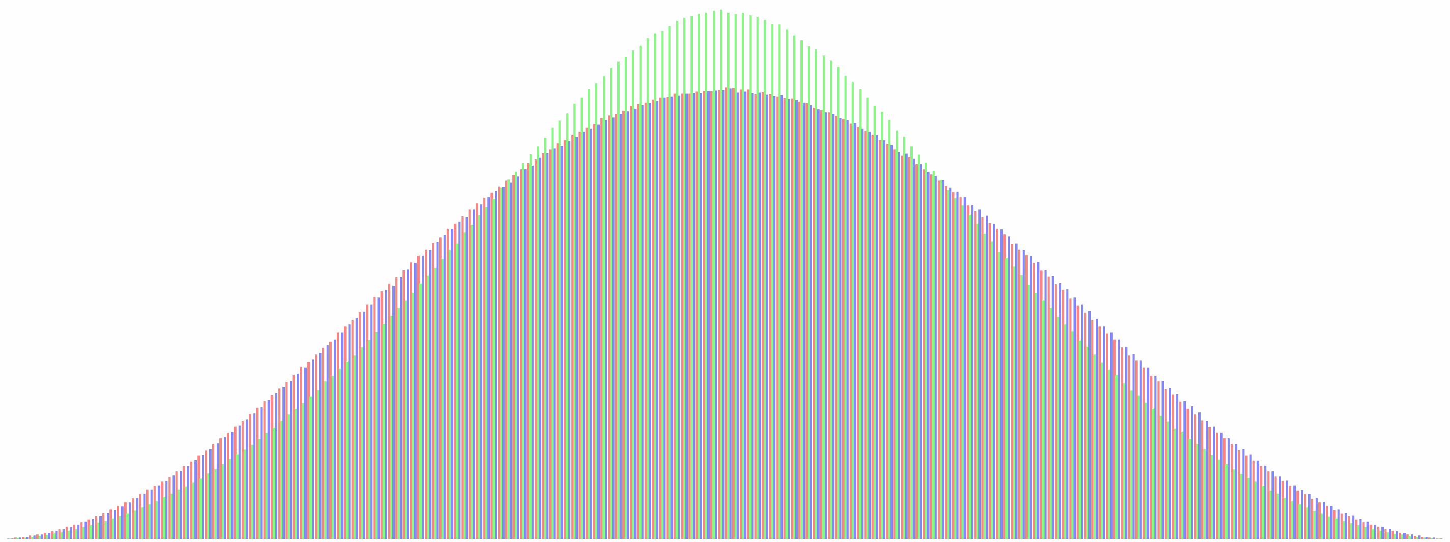
Here are my simulation results: Three generation algorithms each generated 200 million bivectors, and I plotted histograms of the duality distribution of bivectors obtained by the three algorithms. Red corresponds to the “random walk” algorithm superimposing 100 simple bivectors, green corresponds to the algorithm taking logarithms of random rotations, and blue corresponds to the algorithm taking random points on a five-dimensional hypersphere. We can see that the distribution generated by taking logarithms of random rotations is more concentrated toward the middle representing simple bivectors, while the distributions obtained by the other two algorithms are almost identical. We can confirm that the “random walk” algorithm and five-dimensional hypersphere algorithm produce the true uniform distribution.

Why do logarithms of random rotations result in more bias toward simple bivectors? This is because simple bivectors can only generate simple rotations, while compound bivectors can sometimes also generate simple rotations. Consider the rotation generated by the bivector ${11\pi/ 6}e_{xy}+2\pi e_{zw}$: Since $2\pi e_{zw}$ rotates a full circle, equivalent to no rotation, the entire rotation is equivalent to a simple rotation of -30° in the $xy$ direction. Yet this bivector is actually very close to self-dual. When taking logarithms, it only gives the simplest direct generator with rotation angle less than 180 degrees and won’t recover the original compound rotation, thus amplifying the proportion of simple bivectors.

Principal Axis Theorem for Four-Dimensional Rigid Bodies

You might wonder: since four-dimensional rotation has 6 degrees of freedom, this means the moment of inertia has six parameters to describe it (the moment of inertia is a symmetric matrix that can always be diagonalized, thus requiring 6 parameters). But the hyperrectangular box we just discussed has only four dimensions, missing two degrees of freedom. Might we have missed some rotational stability analysis cases? For instance, might there exist shapes even less symmetric than hyperrectangular boxes with more complex rotation patterns? The answer is no. The six parameters of moment of inertia are not independent - the independent degrees of freedom are just 4, and they can all be made equivalent to the moment of inertia of a hyperrectangular box. If readers aren’t interested in specific details, this article ends here. Below I attach the derivation of the four-dimensional rigid body moment of inertia tensor and proof of the principal axis theorem.

Optional Reading 1: Derivation of the Four-Dimensional Moment of Inertia Tensor

Rigid Body Momentum Formula

Let’s first look at the derivation of the rigid body momentum formula as a warm-up. The momentum of a point mass is defined as $p=mv$, where $m$ is the mass and $v$ is the velocity. A rigid body is an aggregate of many point masses, so the total momentum of the rigid body is the sum of all point mass momenta:
$$p=\sum_i m_iv_i$$Define the total mass $m$ as $m=\sum_i m_i$, then the rigid body’s total momentum is equivalent to the weighted average velocity by mass ratio times the total mass:$$p=m\sum_i {m_i\over m} v_i$$Let the rigid body’s average velocity $v$ be$$v=\sum_i {m_i\over m} v_i$$Thus we obtain the rigid body momentum formula as $p=mv$. It’s exactly the same as the point mass momentum formula. Furthermore, according to the properties of the rigid body’s center of mass, we know this average velocity $v$ is precisely the velocity of the center of mass. This property holds in any dimension.

Rigid Body Angular Momentum Formula

Now let’s look at angular momentum. In three-dimensional space, the angular momentum vector of a point mass is defined as$$J=r\times p=mr\times v$$where $r$ is the position of the point mass and $p=mv$ is its momentum. However, we know that four-dimensional space doesn’t have cross products. The direction of angular momentum can no longer be described as along which axis, but rather in which plane, so we need to replace the cross product in the definition with the wedge product:$$J=r\wedge p = m r \wedge v$$The total angular momentum $J$ of a rigid body is the sum of all point mass angular momenta:$$J=\sum_i J_i = \sum_i m_i r_i \wedge v_i$$
Rigid bodies have a characteristic: to maintain rigidity without deformation, the velocities of different parts have mandatory constraint relationships. Specifically, this is reflected in being able to describe the velocity distribution of all point masses using just two global physical quantities - the velocity $v$ at the center of mass $r$ and the angular velocity $\omega$ of rotation around the center of mass:$$v_i=v+(r_i-r).\omega$$Note that the multiplication operation here where position times angular velocity gives linear velocity is no longer cross product but a new kind of “dot product”. The dot product rules are as follows:
$$e_{y}.e_{xy}=-e_{x}$$$$e_{x}.e_{xy}=e_{y}$$$$e_{z}.e_{xy}=0$$where $x$, $y$, $z$ can be letters corresponding to any coordinate axes. This is actually an operation derived from geometric algebra. Readers just need to understand that the angular velocity direction $e_{xy}$ represents rotation in the $xy$ plane from the positive $x$ axis toward the positive $y$ axis to easily verify this is the same as the originally defined angular velocity formula.

Substituting the new velocity relationship into the angular momentum expression, we get
$$J=\sum_i m_i r_i \wedge (v+(r_i-r).\omega)$$
We split this into two terms: the first is orbital angular momentum $L$, the second is spin angular momentum $S$:
$$J=L+S=(\sum_i m_i r_i \wedge v)+(\sum_i m_i r_i \wedge( (r_i-r).\omega))$$
Note that the center of mass $r$ is defined precisely as the mass-weighted average of point positions, so we transform:$$L=m\sum_i {m_i\over m} r_i \wedge v$$It’s easy to see this simplifies to $L=m r \wedge v$, meaning the orbital angular momentum calculation formula is the same as for a single point mass.

The second term, spin angular momentum $S$, is more troublesome:$$S = \sum_i m_i r_i \wedge ((r_i-r).\omega)$$We add a compensating term to convert all position coordinates relative to the center of mass:$$S = \sum_i m_i (r_i-r) \wedge ((r_i-r).\omega) + \sum_i m_i r \wedge ((r_i-r).\omega)$$The added term is actually zero because:$$\sum_i m_i r \wedge ((r_i-r).\omega)=mr\wedge((r-r).\omega)=0$$We can see that the position of the center of mass only affects orbital angular momentum, not spin angular momentum. Therefore, we might as well assume the center of mass is at the origin, and the previous expression can be written as$$S=\sum_i m_i r_i \wedge (r_i.\omega)$$At this step, no further simplification is possible. Let a single point mass have coordinates $r_i=(r_{xi},r_{yi},r_{zi},r_{wi})$. Expanding the wedge and dot products by coordinates through lengthy calculation yields the above expression equivalent to the following matrix expression:
$$S = \mathrm{I}\omega$$where$$\mathrm{I}=\sum_i m_i\begin{pmatrix}r_{xi}^2+r_{yi}^2&r_{yi}r_{zi}&r_{yi}r_{wi}&-r_{xi}r_{zi}&-r_{xi}r_{wi}&0\\r_{yi}r_{zi}&r_{xi}^2+r_{zi}^2&r_{zi}r_{wi}&r_{xi}r_{yi}&0&-r_{xi}r_{wi}\\r_{yi}r_{wi}&r_{zi}r_{wi}&r_{xi}^2+r_{wi}^2&0&r_{xi}r_{yi}&r_{xi}r_{zi}\\-r_{xi}r_{zi}&r_{xi}r_{yi}&0&r_{yi}^2+r_{zi}^2&r_{zi}r_{wi}&-r_{yi}r_{wi}\\-r_{xi}r_{wi}&0&r_{xi}r_{yi}&r_{zi}r_{wi}&r_{yi}^2+r_{wi}^2&r_{yi}r_{zi}\\0&-r_{xi}r_{wi}&r_{xi}r_{zi}&-r_{yi}r_{wi}&r_{yi}r_{zi}&r_{zi}^2+r_{wi}^2\end{pmatrix}$$We treat the bivectors $S$ and $\omega$ as six-dimensional vectors with basis {$e_{xy},e_{xz},e_{xw},e_{yz},e_{yw},e_{zw}$}. That large matrix $\mathrm{I}$ is the so-called four-dimensional moment of inertia matrix. Moment of inertia is a tensor: it’s essentially a linear mapping from angular velocity to angular momentum. The relationship between tensors and matrices is like that between vectors and coordinates: the same tensor will have different matrix forms when different coordinate systems are chosen.

Finally, let’s organize the rigid body angular momentum formula. This formula holds in any dimension, though the inertia matrix becomes increasingly large - its side length grows quadratically with dimension, and total elements grow as the fourth power of dimension. We treat bivectors as second-order tensors, but they’re actually fourth-order tensors.
$$J=L+S=(mr\wedge v)+\mathrm{I}\omega$$

Optional Reading 2: Proof of the Principal Axis Theorem

Principal Axes and Matrix Diagonalization

The moment of inertia of a three-dimensional rectangular box is a diagonal matrix. For general shapes, since the inertia matrix is real symmetric, linear algebra tells us we can always find a rotation transformation $R$ to diagonalize the matrix: $\mathrm{I}’=\mathrm{RIR}^{-1}$, where the rotation matrix $\mathrm{R}$ consists of the eigenvectors of $\mathrm{I}$.
Similarly, we easily know that the moment of inertia of a four-dimensional hyperrectangular box is also a diagonal matrix. We can diagonalize it using the same method:$$\mathrm{I}’=\mathrm{RIR}^{-1}=\mathrm{diag}(I_{xy},I_{xz},I_{xw},I_{yz},I_{yw},I_{zw})$$where $\mathrm{R}$ is a six-dimensional orthogonal matrix composed of eigenvectors of $\mathrm{I}$, and $I_{ij}$ are the corresponding eigenvalues.
But note that the matrix is now six-dimensional. Even after obtaining the transformation matrix $R$, it’s an orthogonal transformation in six-dimensional bivector space. But four-dimensional rotation has 6 degrees of freedom while six-dimensional rotation has 15 degrees of freedom, so the orthogonal transformation found in six-dimensional space may not correspond to a valid four-dimensional space rotation. The problem seems stuck here.

Inertia Matrix in Isoclinic Coordinates

From the matrix expression of moment of inertia, we can discover some patterns, such as the matrix being symmetric and the anti-diagonal elements always being 0 (caused by absolutely perpendicular rotations not affecting each other). We also know that left and right isoclinic rotations don’t interfere with each other, which suggests that if we transform to an “isoclinic coordinate system,” the moment of inertia matrix form might decouple into smaller block matrices for processing, thus obtaining more properties of moment of inertia. Decoupling also has the benefit of reducing the dimension of matrices needed for principal axis diagonalization, eliminating redundant degrees of freedom, perhaps avoiding the previous predicament.

We transform the original bivector’s six coordinate plane basis$$e_{xy},e_{xz},e_{xw},e_{yz},e_{yw},e_{zw}$$into a basis of three self-dual and three anti-self-dual unit bivectors:$${\sqrt 2\over 2}(e_{xy}+e_{zw}),{\sqrt 2\over 2}(e_{xz}-e_{yw}),{\sqrt 2\over 2}(e_{xw}+e_{yz}),{\sqrt 2\over 2}(e_{xy}-e_{zw}),{\sqrt 2\over 2}(e_{xz}+e_{yw}),{\sqrt 2\over 2}(e_{xw}-e_{yz})$$In the new coordinate system, the moment of inertia matrix $\mathrm{I}$ becomes
$$\mathrm{I}’=\sum_i m_i\begin{pmatrix}
\frac{1}{2}(r_{xi}^2+r_{yi}^2+r_{zi}^2+r_{wi}^2)&0&0&\frac{1}{2}(r_{xi}^2+r_{yi}^2-r_{zi}^2-r_{wi}^2)&r_{yi}r_{zi}-r_{xi}r_{wi}&r_{xi}r_{zi}+r_{yi}r_{wi}\\0&\frac{1}{2}(r_{xi}^2+r_{yi}^2+r_{zi}^2+r_{wi}^2)&0&r_{xi}r_{wi}+r_{yi}r_{zi}&\frac{1}{2}(r_{xi}^2-r_{yi}^2+r_{zi}^2-r_{wi}^2)&r_{zi}r_{wi}-r_{xi}r_{yi}\\0&0&\frac{1}{2}(r_{xi}^2+r_{yi}^2+r_{zi}^2+r_{wi}^2)&r_{yi}r_{wi}-r_{xi}r_{zi}&r_{xi}r_{yi}+r_{zi}r_{wi}&\frac{1}{2}(r_{xi}^2-r_{yi}^2-r_{zi}^2+r_{wi}^2)\\\frac{1}{2}(r_{xi}^2+r_{yi}^2-r_{zi}^2-r_{wi}^2)&r_{xi}r_{wi}+r_{yi}r_{zi}&r_{yi}r_{wi}-r_{xi}r_{zi}&\frac{1}{2}(r_{xi}^2+r_{yi}^2+r_{zi}^2+r_{wi}^2)&0&0\\r_{yi}r_{zi}-r_{xi}r_{wi}&\frac{1}{2}(r_{xi}^2-r_{yi}^2+r_{zi}^2-r_{wi}^2)&r_{xi}r_{yi}+r_{zi}r_{wi}&0&\frac{1}{2}(r_{xi}^2+r_{yi}^2+r_{zi}^2+r_{wi}^2)&0\\r_{xi}r_{zi}+r_{yi}r_{wi}&r_{zi}r_{wi}-r_{xi}r_{yi}&\frac{1}{2}(r_{xi}^2-r_{yi}^2-r_{zi}^2+r_{wi}^2)&0&0&\frac{1}{2}(r_{xi}^2+r_{yi}^2+r_{zi}^2+r_{wi}^2)\end{pmatrix}
$$This matrix is quite large, but it can indeed be written as a block matrix:
$$\mathrm{I}’=\begin{pmatrix}
\lambda \text{I}_{3\times 3} & \text{P} \\ \text{P}^T & \lambda \text{I}_{3\times 3}
\end{pmatrix}$$where $\lambda=\frac{1}{2}\sum_i m_i(r_{xi}^2+r_{yi}^2+r_{zi}^2+r_{wi}^2)$, and $\text{P}$ is typically a non-symmetric third-order matrix. What happens if the original matrix is diagonal when transformed to isoclinic coordinates? Let$$\mathrm{I}_1=\mathrm{diag}(I_{xy},I_{xz},I_{xw},I_{yz},I_{yw},I_{zw})$$Transforming it to isoclinic coordinates yields$$\mathrm{I}’_1=\frac{1}{2}\begin{pmatrix}I_{xy}+I_{zw}&0&0&I_{xy}-I_{zw}&0&0\\0&I_{xz}+I_{yw}&0&0&I_{xz}-I_{yw}&0\\0&0&I_{xw}+I_{yz}&0&0&I_{xw}-I_{yz}\\I_{xy}-I_{zw}&0&0&I_{xy}+I_{zw}&0&0\\0&I_{xz}-I_{yw}&0&0&I_{xz}+I_{yw}&0\\0&0&I_{xw}-I_{yz}&0&0&I_{xw}+I_{yz}\end{pmatrix}$$Comparing with the previous $\mathrm{I}’$ matrix expression, we know that elements on the main diagonal in isoclinic coordinates must be equal, thus$$I_{xw}+I_{yz}=I_{xy}+I_{zw}=I_{xw}+I_{yz}$$From this we can see that although the diagonalized sixth-order matrix has six degrees of freedom, the geometric properties of moment of inertia reduce these degrees of freedom to just 4 - only the four dimensions of the hyperrectangular box remain. To prove the principal axis theorem, only one final step remains: prove that any matrix $\mathrm{I}’$ can be transformed through four-dimensional space rotation into the form $\mathrm{I}’_1$. Comparing $\mathrm{I}’$ with $\mathrm{I}’_1$, we see that the original diagonal matrix is no longer diagonal when converted to isoclinic coordinates, but becomes a block matrix where submatrix $\mathrm P$ in $\mathrm{I}’$ is also diagonal. We just need to find an appropriate rotation transformation to diagonalize $\text{P}$ to find the transformation to the principal axis coordinate system.

Solving the Four-Dimensional Rotation Transformation

A rotation transformation in four-dimensional space acting on bivectors is also equivalent to a six-dimensional matrix. Its form in isoclinic coordinates is very simple: Due to the commutativity of left and right isoclinic rotations, any four-dimensional bivector rotation matrix transformed to the isoclinic coordinate system becomes a block matrix containing two third-order orthogonal matrices ($\text{A}$, $\text{B}$):
$$\text{R}=\begin{pmatrix}
\text{A} & 0 \\ 0 & \text{B}
\end{pmatrix}$$We need this rotation matrix to transform matrix $\text{P}$ into some diagonal matrix $\Lambda$:$$\begin{pmatrix}
\text{A} & 0 \\ 0 & \text{B}
\end{pmatrix} \begin{pmatrix}
\lambda \text{I}_{3\times 3} & \text{P} \\ \text{P}^T & \lambda \text{I}_{3\times 3}
\end{pmatrix} \begin{pmatrix}
\text{A}^T & 0 \\ 0 & \text{B}^T
\end{pmatrix} =\begin{pmatrix}
\lambda \text{I}_{3\times 3} & \Lambda \\ \Lambda & \lambda \text{I}_{3\times 3}
\end{pmatrix}$$
Computing the matrix multiplication on the left and comparing both sides of the equation yields $\Lambda=\text{AP} \text{B}^T$. Since $\text{A}$ and $\text{B}$ are both orthogonal matrices, we can solve for $\text{A}$ and $\text{B}$ using the classic singular value decomposition algorithm. After solving, we obtain the complete four-dimensional bivector rotation matrix $\text{R}$ in the isoclinic coordinate system.

Note that matrix $\text{R}$ is sixth-order, so we still need to find the original four-dimensional rotation matrix or the rotor/quaternion representation of the rotation. The most elegant way is to complete this conversion directly in the isoclinic coordinate system: The orthogonal matrices $\text{A}$ and $\text{B}$ actually represent the left and right isoclinic rotation parts of this rotation. Converting these third-order orthogonal matrix representations of rotations directly to quaternion representations gives the quaternion representation of the entire rotation. The final thing to note is that due to the order issue of quaternion right multiplication, matrix B needs to be transposed once before mapping to quaternions. Conveniently, the $\text A$ and $\text B^T$ obtained from singular value decomposition can be directly converted to left and right multiplying quaternions respectively to get the final quaternion rotor representation of the four-dimensional rotation.