2D Time World

// Note 1: This article is a fictional physical space constructed by the author's own imagination, full of loopholes, for entertainment purposes only, please do not take it seriously.

// Note 2: The 2D time in this article is isotropic, different from the 2D time setting in Greg Egan's "Dichronauts", which we will explore another time.

// Note 3: Some sections in this article may be filled with difficult formulas. I have marked them as optional reading and with colors; you can skip them directly if you are not interested.

What is 2D Time

In this article, we will imagine what a universe with 2D time would look like. For our linear view of spacetime, we believe that a “living” universe needs to change with one parameter. But from the perspective of spacetime, as long as the time trajectories of all particles (called the particles’ world lines) are drawn, the evolution is fixed. So time is just something subjective. In 2D time, particles no longer have world lines but world sheets — the trajectory of each particle in spacetime becomes a 2D surface. In our eyes, 2D spacetime is just some “dead” surfaces solved from physical equations. But perhaps those creatures would naturally feel that time flows on the surface, and it would still be a “living” universe with “dynamics”. What interesting things would happen if the inhabitants of that spacetime naturally believe that time is 2D?

The most significant difference between 2D time and our 1D time is the destruction of causality. Only 1D spacetime can naturally define the sequential relationship of events. Under 2D time, the sequential relationship no longer exists, and there is no strict distinction between past and future. Some might say: 2D time means we can go in circles on a particle’s world sheet, which is like you bringing a magical object back from the future via a time machine, so the object appears in spacetime out of nothing! Actually, this view is a one-sided perspective of the 1D time — for creatures in 2D time, time is an integrated whole and should not be understood by the way we are thinking in our 1D time. Their evolution does not mean selecting a certain world line on the plane, nor does it mean infinite world lines constituting a “parallel universe”. Instead, it unfolds in “all directions” on the 2D time coordinate surface. Selecting a special time line is similar to how we might view a 2D cross-section of a 3D object — possible but unnatural.

Another significant difference is that for them, the concepts of past and future may not even be needed. It is even difficult for us to tell stories about their world because our hearing is linear, while their storyline is more like a map. You might ask, what is their “memory” like? Can they perceive the entire history of spacetime? Perhaps readers will have the answer after finishing this article. Let us first sort out the axioms and possibly “reasonable” physical laws in this universe. If you are not interested in the specific physical details, please skip to the Ball Collision Simulation section.

Notation Conventions

Unless otherwise specified in this article, 2D time spacetime specifically refers to a 5D spacetime obtained from 3D space (x/y/z) plus 2D time (u/v), i.e., a spacetime with the following metric: $$\mathrm{d}s^2 = \mathrm{d}x^2+\mathrm{d}y^2+\mathrm{d}z^2 - \mathrm{d}u^2 - \mathrm{d}v^2$$ Note: Here the letters u and v are used specifically to denote the 2D time, and t is no longer used to break free from the influence of the 1D view of time.

Point Particle Kinematics

In normal 4D spacetime (3D space + 1D time), the world line of a particle at rest relative to a reference frame is a straight line parallel to the time t-axis, while a particle in uniform motion has a slanted line. Therefore, we assume that in 2D time spacetime, the world sheet of a particle at rest relative to a reference frame is a plane parallel to the time coordinate plane uv, and uniform motion corresponds to an inclined plane. How should the velocity of a particle be defined? The usual middle-school definition is displacement per unit time, while the definition in relativistic spacetime is the tangent vector of the world line. Both definitions can be generalized to 2D time, and I will put the latter in optional reading.

Velocity

In our spacetime, the position of a particle is a 3D vector, which is a function of time, denoted as $\vec{\mathbf{r}}(t)$. Its rate of change with respect to the time parameter is naturally the velocity, i.e., $\vec{\mathbf{v}}(t) =\frac{\mathrm{d}\vec{\mathbf{r}}(t)}{\mathrm{d}t}$. In 2D time, the position of a particle is still a 3D vector, but it is a binary function of time, denoted as $\vec{\mathbf{r}}(u,v)$. Its derivatives are more numerous: the rates of change along different time directions can be different. Generally speaking, we need a matrix (tensor) to represent it, i.e., $$\mathbf{v}(u,v) = (\vec{\mathbf{v}}_u,\vec{\mathbf{v}}_v)= \left( \frac{\partial \vec{\mathbf{r}}}{\partial u},\ \frac{\partial \vec{\mathbf{r}}}{\partial v} \right).$$ Note that $\vec{\mathbf{r}}$ itself is a 3D column vector, so the whole thing is a $2\times3$ matrix. For example, the general kinematic equation for uniform motion of a particle is $$\vec{\mathbf{r}}(u,v) = (\mathrm{v}_{xu} u + \mathrm{v}_{xv} v, \mathrm{v}_{yu} u + \mathrm{v}_{yv} v, \mathrm{v}_{zu} u + \mathrm{v}_{zv} v)$$ The velocity of the particle is constantly: $$\mathbf{v} = \begin{pmatrix} \mathrm{v}_{xu} & \mathrm{v}_{xv} \\ \mathrm{v}_{yu} & \mathrm{v}_{yv} \\ \mathrm{v}_{zu} & \mathrm{v}_{zv} \end{pmatrix}$$
Similarly, acceleration is a higher-order $2\times2\times3$ tensor, which will be introduced in the next section.

Optional Reading: Bivector Version of Velocity

Next, let’s look at the velocity of a particle again from the perspective of world sheets in spacetime.
In our Newtonian mechanics, velocity can be viewed as the spatial part of the tangent vector of the world line when its time component is scaled to 1. This is equivalent to the description of displacement per unit time. In 2D time, the tangent object at a point on a world sheet is no longer a vector but a 2D surface-like bivector. If you are unfamiliar with this kind of vector, please refer to 4D Space (VII): N-Dimensional Vectors. Specifically, this is a tangent plane bivector in 5D spacetime, which may have components: $e_x\wedge e_y$, $e_x\wedge e_z$, $e_x\wedge e_u$, $e_x\wedge e_v$, $e_y\wedge e_z$, $e_y\wedge e_u$, $e_y\wedge e_v$, $e_z\wedge e_u$, $e_z\wedge e_v$, $e_u\wedge e_v$. In the non-relativistic low-speed approximation, if the coefficient of the pure time component $e_u\wedge e_v$ is scaled to 1, then the other components describe the particle’s velocity. We can specifically compute the bivector version of the velocity for $\mathbf{v}(u,v)=(\vec{\mathbf{v}}_u,\vec{\mathbf{v}}_v)$. By definition, this bivector is clearly spanned by $\mathbf{T}_u = (\vec{\mathbf{v}}_u,\ 1,\ 0)$ and $\mathbf{T}_v = (\vec{\mathbf{v}}_v,\ 0,\ 1)$. Their exterior product gives the bivector: $$ \begin{aligned}
\mathbf{B} &= \left(\vec{\mathbf{v}}_u + \mathbf{e}_u \right) \wedge \left(\vec{\mathbf{v}}_v+\mathbf{e}_v \right) \\
&= \mathbf{e}_u \wedge \mathbf{e}_v + \vec{\mathbf{v}}_u\wedge \mathbf{e}_v - \vec{\mathbf{v}}_v\wedge \mathbf{e}_u +\vec{\mathbf{v}}_u\wedge\vec{\mathbf{v}}_v
\end{aligned}
$$ Expanding in components gives: $$\mathbf{B} = \mathbf{e}_u \wedge \mathbf{e}_v + \sum_i \left( \mathrm{v}_{iu} \mathbf{e}_i \wedge \mathbf{e}_v - \mathrm{v}_{iv} \mathbf{e}_i \wedge \mathbf{e}_u \right) + \sum_{i < j} (\mathrm{v}_{iu} \mathrm{v}_{jv} - \mathrm{v}_{iv} \mathrm{v}_{ju}) \mathbf{e}_i \wedge \mathbf{e}_j $$ Here the first term, the pure time component, is already unit 1, which is great; the second term represents the spacetime components of velocity, which is exactly the information we want to describe the particle’s velocity; but the third term is a purely spatial component. What are these things? It is actually the exterior product of the two velocities, which can be seen as the “area” traversed by a particle per unit time: imagine a particle moving along the $x$-axis in the $u$ direction and along the $y$-axis in the $v$ direction. Its velocity matrix is: $\begin{pmatrix} 1 & 0 \\ 0 & 1 \\ 0 & 0 \end{pmatrix}$, and the velocity bivector is: $\mathbf{e}_u\wedge\mathbf{e}_v + \mathbf{e}_x\wedge\mathbf{e}_v + \mathbf{e}_y\wedge\mathbf{e}_u + \mathbf{e}_x\wedge\mathbf{e}_y$. The projection of the world sheet in xyz space per unit area of time is this $\mathbf{e}_x\wedge\mathbf{e}_y$.

Uniformly Accelerated Motion

Consider a particle in free fall in a gravitational field. What would this scenario look like in 2D time? In our world, uniformly accelerated motion is defined as: $\vec{\mathbf{v}} = \vec{\mathbf{a}} t$. In 2D time, this is decomposed into $$\vec{\mathbf{v}}_u = \vec{\mathbf{a}}_{uu} u + \vec{\mathbf{a}}_{uv} v, \qquad \vec{\mathbf{v}}_v = \vec{\mathbf{a}}_{vu} u + \vec{\mathbf{a}}_{vv} v.$$ Since acceleration comes from the second-order partial derivatives of the same position function $\vec{\mathbf{r}}(u,v)$, by the commutativity of mixed partial derivatives we have $\vec{\mathbf{a}}_{uv}=\vec{\mathbf{a}}_{vu}$, meaning the acceleration tensor must be symmetric. Written as a matrix: $$\begin{pmatrix}\vec{\mathbf{v}}_u \\
\vec{\mathbf{v}}_v
\end{pmatrix}=\begin{pmatrix}
\vec{\mathbf{a}}_{uu} & \vec{\mathbf{a}}_{uv} \\
\vec{\mathbf{a}}_{vu} & \vec{\mathbf{a}}_{vv}
\end{pmatrix}
\begin{pmatrix}
u \\ v
\end{pmatrix}$$ All four acceleration components are 3D vectors, so we say acceleration is a $2\times2\times3$ order tensor.

Assume this planet has a gravitational acceleration $g$ pointing along the $x$-axis, and it affects the time $u$ and $v$ equally, i.e., $\vec{\mathbf{a}}_{uu} = \vec{\mathbf{a}}_{vv} = g\vec{\mathbf{e}}_x$, $\vec{\mathbf{a}}_{uv} = \vec{\mathbf{a}}_{vu} = \mathbf{0}$. Suppose at the given time $u=0, v=0$ the particle is at the origin, with initial velocities $\vec{\mathbf{v}_u}(0)$ and $\vec{\mathbf{v}_v}(0)$. It is easy to solve: $$\vec{\mathbf{r}}(u,v) = u \vec{\mathbf{v}}_u(0) + v \vec{\mathbf{v}}_v(0) + \frac{1}{2}g\left(u^{2}+v^{2}\right)\vec{\mathbf{e}}_x$$ Here we see that for a particle with a given constant acceleration, we only need the initial position and initial velocity at one time, just like in 1D time, and the entire motion state over the whole time region can be solved. Moreover, can all general uniformly accelerated motions be diagonalized by choosing a reference frame to eliminate cross terms? The answer is no: the acceleration matrix is symmetric. A classic result from linear algebra says that real symmetric matrices can be diagonalized via rotations. This means that, generally speaking, it is impossible to simultaneously diagonalize the three component matrices (x, y, z) with one rotation.

Reference Frame Transformations

In 2D time spacetime, ignoring relativity, the Galilean spacetime symmetries include spatial rotations, rotations within the time plane, and velocity transformations between space and time. Together they form the Galilean transformation group. We want all physical laws to remain invariant under these three transformations:

1. Spatial Rotation
   This part is just the usual spatial rotation transformation in xyz, meaning that all directions in space are equivalent, with no preferred direction, and any direction can serve as a coordinate axis.
2. Velocity transformation (Boost)
   A particle can move uniformly along the two time directions separately. The following reference frame transformation (called boost) can keep the particle at rest relative to the new coordinates: $$\vec{\mathbf{r}}’ = \vec{\mathbf{r}} - \vec{\mathbf{v}}_u u - \vec{\mathbf{v}}_v v,$$ where $\vec{\mathbf{v}}_u,\vec{\mathbf{v}}_v$ are constant vectors representing the relative velocities between the old and new reference frames along the time parameter $u$ and time parameter $v$ respectively. Written in matrix form: $$
   \begin{pmatrix} x’ \\ y’ \\ z’ \end{pmatrix}=\begin{pmatrix} x \\ y \\ z \end{pmatrix} -\begin{pmatrix} \mathrm{v}_{xu} & \mathrm{v}_{xv} \\ \mathrm{v}_{yu} & \mathrm{v}_{yv} \\ \mathrm{v}_{zu} & \mathrm{v}_{zv}\end{pmatrix}\begin{pmatrix} u \\ v \end{pmatrix} $$
3. Time Rotation
   This is a brand new reference frame transformation that does not exist in 1D time. Since the two time parameters have equal status, the uv time plane has rotational symmetry, and rotations preserve $u^2+v^2$: $$\begin{pmatrix} u’ \\ v’ \end{pmatrix}=\begin{pmatrix} \cos\theta & -\sin\theta \\ \sin\theta & \cos\theta \end{pmatrix}\begin{pmatrix} u \\ v \end{pmatrix}$$

Newton’s Second Law

Next, let’s study particle dynamics. We need to generalize Newton’s laws. The third law is straightforward and can continue to hold; the first law is a special case of the second law, so we directly discuss the form of the second law: If we directly transplant Newton’s second law into 2D time, letting force equal mass times the acceleration tensor, then force is also a $2\times2\times3$ tensor: $\vec{\mathbf{F}}_{\alpha\beta} = m \vec{\mathbf{a}}_{\alpha\beta}$ (indices take $u$, $v$). This seems self-consistent, but there are difficulties: if force completely determines acceleration, the particle in the uniformly accelerated motion solution above shows that the particle’s state at one instant determines the entire world sheet of the particle. Even worse, consider a particle that is only acted on by a force in a finite time region. Outside that region, there is no force, and the acceleration tensor is entirely zero, meaning the world sheet must be a plane outside that region. The influence of the force is completely confined within the region where it acts and cannot propagate to the outside. This would make the effect of forces in finite time regions, such as particle collisions, meaningless.

Another approach is to adopt a different generalization of Newton’s second law. Here we choose to use the Lagrangian from analytical mechanics to derive the particle’s dynamical equations. It doesn’t matter if you don’t understand; we only need the conclusion.

(Optional Reading) Define the Lagrangian density of a particle as $$ \mathcal{L} = \frac12 m\bigl( |\partial_u\vec{\mathbf{r}}|^2 + |\partial_v\vec{\mathbf{r}}|^2 \bigr) - V(\vec{\mathbf{r}}) $$ The action is the double integral over the time plane $S = \iint \mathcal{L} \mathrm{d}u \mathrm{d}v$. Varying $\vec{\mathbf{r}} \to \vec{\mathbf{r}}+\delta\vec{\mathbf{r}}$ and integrating by parts gives the following equation of motion:

$$ \vec{\mathbf{F}}= m\Bigl( \frac{\partial^2\vec{\mathbf{r}}}{\partial u^2} + \frac{\partial^2\vec{\mathbf{r}}}{\partial v^2} \Bigr) $$ Here the external force can be the gradient of potential $-\nabla V$, which is still the familiar vector, and it only couples to the trace of the acceleration tensor (the sum of the two second derivatives). The remaining independent components of acceleration are not constrained by the force.

Newton’s First Law

Setting the force on the right-hand side to zero gives the equation of motion for a free particle, which is the 2D Laplace equation $$ \frac{\partial^2\vec{\mathbf{r}}}{\partial u^2} + \frac{\partial^2\vec{\mathbf{r}}}{\partial v^2} = \mathbf{0}, $$ That is, the particle’s world sheet resembles a minimal surface, and each position coordinate of the particle is a harmonic function on the time plane. This means that even without a force, the world sheet need not be a plane; it can bend according to given boundary conditions in time. This perfectly solves the previous problem: our familiar initial value problem requires specifying the position and velocity distribution along an entire initial time line, not just at a single point. This reflects the greater degrees of freedom predicted by 2D time physics. If we instead force the force to be proportional to a particular acceleration vector to eliminate the multiple solutions, we would actually obliterate these rich structures.

Other Possible Choice?

From the perspective of spacetime geometry, Newtonian mechanics with 1D time has force equal to curvature of curves, while with 2D time it has force equal to mean curvature of surfaces. Some readers might wonder why force should correspond to mean curvature; what if we used Gaussian curvature instead? In 1D time, a particle’s geodesic never has Gaussian curvature, so this is not a good analogy. Readers might also consider other different forms of Newton’s second law. However, the simplest form that keeps the energy positive definite while preserving rotational symmetry in the 2D time plane is this one. Therefore, we will not dwell further on why Newton’s second law is set up this way.

Ball Collision Simulation

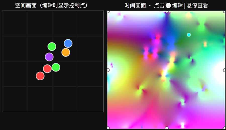
I wrote a simple simulator: 2D2T, with the help of AI, for ball collisions in 2D space + 2D time. It has features such as setting boundary conditions, editing positions of multiple balls, solving the Laplace equation, simulating gravity and collision repulsion, and hovering over time points to view the state of balls in space. However, the collisions between balls and between balls and walls are still not quite correct: I saw the AI uses averaging over neighboring time points to iteratively solve the Laplace equation, which is OK yet. But for external forces (such as applying a downward gravity force), it directly adds a small downward displacement to the balls and then uses boundary conditions to smooth the solution. However, this pulls the space downward under gravity, and with the boundary fixed, it stretches the space into a “bag” shape. The Laplacian at the middle of this bag has a positive sign, meaning the force is actually upward. It seems the direction of the force is reversed. When simulating collisions between balls, along a certain time line it also looks like the balls attract each other, get close, and then are thrown apart. Therefore, I directly reversed the direction of the force, but this causes the collision simulation to diverge. Thus, rather than ball collisions, this scenario is more like an N-body system of mutually attracting celestial bodies with restricted gravitational range. But currently, I have not found an algorithm that can stably solve 2D time collisions. This vibe-coded simulator can only be taken as entertainment.

I also discovered an interesting phenomenon: replacing the RGB color channels with the velocity magnitude |V| of different balls, one can see that near some time points the balls have very high speeds, and the coloring looks like individual dipoles. These instants correspond to time periods when balls are very close to each other and quickly pass by. That is, the set of moments when balls attract and meet forms zero-dimensional points on the uv plane, rather than a 1D line. During iteration, I also found that some nearby passing points can get closer to each other with iteration and eventually merge and disappear. I am not sure why. It should be noted that the merging and disappearance of passing points occurs during the solver iteration; it is not a state evolution in 2D time, but just an intermediate result of the computation. So this phenomenon actually has no physical meaning.

It should also be particularly pointed out here that although we first determined the positions of the balls on the time-plane boundary and then iteratively solved for all states of the balls in spacetime, the “history” of the entire 2D universe is laid out all at once. As long as every point in spacetime satisfies the relevant dynamical equations, it is fine. For creatures in 2D time, they only know the states near their own time point. In their view, time evolution spreads outward from the center into the unknown, rather than the reverse: from the determined exterior (boundary) inward.

Entropy and the Arrow of Time

The fact that our time has a one-way direction is closely related to the direction of entropy. In ordinary 1D time, given an initial state, the mechanical equations determine the future. But in fact, all physical laws have time-reversal symmetry: throwing a basketball and catching it, when played in reverse, still shows throwing and catching. But systems involving thermodynamic losses cannot be reversed, e.g., a bouncing ball on the ground recovers to a lower height each time; in reverse, we would see the ball bouncing higher and higher, which is impossible in reality. A mirror falling to the floor and shattering, when played in reverse, shows the impossible event of a broken mirror reuniting. The principle of increasing entropy asserts that for macroscopic systems, the number of future states (entropy, or probability) is far greater than the past. In fact, we even directly use the direction of increasing entropy (increasing probability) as the definition of the future direction of time.

The coin-flipping model can help us understand entropy simply: suppose initially there are $N$ coins with heads facing up. Each step, randomly select one coin and flip it. Over time, the number of heads will approach $N/2$. However, this is a random process; it won’t just keep approaching $N/2$ monotonically but will fluctuate randomly. After reaching near $N/2$, it will continue to fluctuate, and it might even return to the state where all coins are heads up. Of course, if $N$ is slightly larger, the waiting time to return to the all-heads state increases exponentially, possibly taking longer than the lifetime of the universe. For more information, search online for the keyword: Poincaré recurrence.

How can entropy be defined in 2D time? We have already constructed a bunch of particles with collisions (whether repulsive or attractive doesn’t matter; it’s the interaction). The particle distribution at each moment will naturally have disorder and order, and the concept of entropy can also be defined. A 2D time system has no intrinsic direction of evolution — all history is “laid out at once” on the time plane as world sheets. Therefore, we can take a different perspective: treat entropy as a field distributed on the 2D time plane. We can imagine that the entropy function on the time plane undulates like terrain. The direction of entropy increase is naturally the gradient direction of the terrain. 2D beings might be able to perceive a specific 1D arrow of time, and these arrows of time might flow down the slopes like rainwater, converging and eventually flowing into the low-lying ocean of heat death. If we still want to use the random coin-flipping model to simulate the evolution of a 2D time system, we would require that the two coins flipped from time (0,0) to (0,1) to (1,1) are the same as those from (0,0) to (1,0) to (1,1). In this way, each step’s random coin flip has strong correlations, rather than being completely random. I asked an AI to write a 2D time entropy simulator — EN2T: First, set the number of coins $N$. At each time, these $N$ parameters can be either 0 or 1. In traditional 1D time, at $t=0$, all parameters are 0, and then at the next moment, one coin’s 0/1 state is randomly flipped. In the 2D time version, time is discretized into a grid. At the initial selected time (u,v)=(0,0), between any two adjacent moments (only four neighbors, not diagonal), at most one coin state can differ. 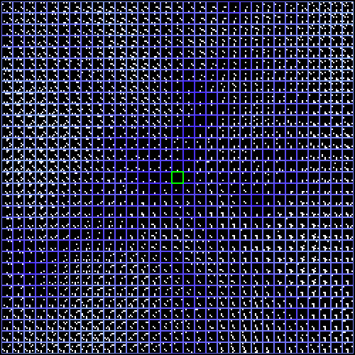How can we obtain a random state distribution as much as possible under such constraints? I used a greedy algorithm, letting the grid states “grow” like crystal nuclei. Suppose we select an undetermined grid point that has neighbors with determined states:

• If there is exactly one neighbor with a determined state, copy that neighbor’s state and randomly flip one coin;
• If there are two neighbors with determined states and both are identical, still randomly flip one coin;
• If there are two neighbors with determined states and they are not identical, there are two subcases:
  1. Only one coin state differs: randomly choose one of the two neighbor states and copy it;
  2. Exactly two coin states differ: denote the two different coins as a and b, copy the state of the first neighbor, then randomly choose either a or b and flip it.

If we can ensure that there are never three or more determined neighbors during the process, this algorithm can generate completely consistent solutions without backtracking. Therefore, the order in which we traverse the undetermined grid points is very important. I first used a square spiral traversal and found that the state changes significantly more slowly along the diagonal direction. Later, I improved it by adding some randomness, but it still left obvious radial stripes. I think this is a problem with the greedy algorithm. If a more complex strategy with backtracking were used, it should be possible to achieve a completely random distribution on the plane. And our model already shows that the distribution of entropy in 2D time can indeed undulate like terrain.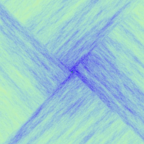


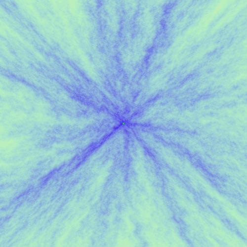
You might feel a bit disappointed that 2D time has turned into traditional 1D time again. But I want to say that these arrows of time might not strictly separate the past and future like traditional 1D time: although there may be a single overall thermodynamic evolution trend, local rotational symmetry in time still exists. I speculate that the memory of 2D-time creatures is like this: they can remember the entire region not far from their time point, but as the time distance increases, the memory gradually fades, and eventually becomes completely imperceptible. This memory decay here is different from our forgetting. Forgetting is merely an active mechanism of losing memory by living beings. Even if written on paper or in computers, these storage media will also “forget.” Their memory decay is determined by the physical and geometric factors of time.

The following sections are more technical. If readers are not interested in formulas, you can directly click here to jump directly to the electromagnetic wave simulator section.

Optional Reading: Relativistic Formulation of Force

In the relativistic 5D spacetime $\mathbb{R}^{3,2}$, the history of a particle is a 2D world sheet $\Sigma$. The tangent plane of the world sheet can be represented by a unit 2-form field $\Omega^{ab}$ (i.e., the antisymmetric tensor corresponding to the bivector of the tangent plane, using abstract index notation). It satisfies:

• Antisymmetry: $\Omega^{ab}=-\Omega^{ba}$
• Normalization: $ \Omega^{ab}\Omega_{ab} = 2$
• Simplicity: $\Omega^{[ab}\Omega^{cd]} = 0$

Analogous to the acceleration vector $a^a = u^b\nabla_b u^a$ in the 1D time world, the equation of motion for a particle in the 2D time world can be fully formulated using $\Omega^{ab}$ and its covariant derivatives. Combining this with the expression for the mean curvature vector in differential geometry, Newton’s second law can be written as $$ m \Omega^{bc} \nabla_b\Omega^a{}_c = -\mathrm{F}^a $$ where $\mathrm{F}^a$ is the external force density. The form of the left-hand side automatically ensures that the force satisfies the normal condition $\mathrm{F}^a \Omega^b{}_a=0$, i.e., it is perpendicular to the world sheet. Free motion $(\mathrm{F}^a=0)$ is then $$ \Omega^{bc} \nabla_b\Omega^a{}_c = 0 $$

This formulation does not depend on the choice of parameters on the world sheet and is entirely given by the spacetime geometric quantity $\Omega^{ab}$. Readers can verify that in the low-speed approximation, the particle equation of motion reduces to the non-relativistic form given earlier.

Optional Reading: Continuity Equation

We have studied the motion of point particles, or balls. Now let’s look at the motion of general matter: matter is not concentrated at points; it is distributed in the world according to densities. In our world, we have concepts like mass density, charge density, etc., and the continuity equation: $$\frac{\partial\rho}{\partial t} + \nabla\cdot\mathbf{J} = 0$$ This can be understood intuitively as: the total flux of water flowing into a closed surface per unit time equals the mass of water newly added inside that closed surface.

The continuity equation in our 4D spacetime essentially says: the number of particle world lines entering a closed surface in spacetime equals the number exiting. This means that no world lines terminate or are newly created within the closed surface, embodying the conservation of mass. Using a vector field to represent particle density, the above statement is equivalent to the flux of the vector field through a closed surface $\Sigma$ being zero: ($\Sigma_a$ is the (co)normal vector on the closed surface) $$\oint_{\Sigma} J^a \mathrm{d}\Sigma_a = 0$$ Or equivalently, the divergence of the matter flow density field in spacetime is zero: $$\partial_a J^a = 0$$

What does the continuity equation look like for matter in 2D time? We can imagine a 2D-time version of a water pool: the increase or decrease of mass in a closed region with respect to each time parameter (described by partial derivatives) corresponds to an inflow. These two flows are exactly the matter’s velocity field ($\mathbf{v}_u$, $\mathbf{v}_v$) multiplied by the density. $$\frac{\partial\rho}{\partial u} = \nabla\cdot\mathbf{J}_u$$$$\frac{\partial\rho}{\partial v} = \nabla\cdot\mathbf{J}_v$$

The Continuity Equation in Spacetime

Does this equation equivalently describe the continuity of matter? Intuitively, continuous matter distribution in 2D time corresponds to many world sheets in spacetime, layered like pages filling the entire spacetime. Now we use a bivector field $J$ to represent the density of this page-like structure, just as we use a vector field to represent the density of hair-like 1D world lines. We do not want a world sheet to be incomplete, as that would mean a particle disappears in some time region. Let the spatial dimension be N, then the entire spacetime is N+2 dimensional. I initially made some erroneous attempts, First, I thought this: each world sheet intersects the boundary (an N+1 dimensional surface) of a region in N+2 dimensional spacetime along a loop. To capture whether the loop is incomplete, my idea was to add up all the tangent vectors along the loop. If the particle beam is conserved, the sum of vectors around the loop would just be zero. If the density is lower in some region, the balance is broken. However, only scalars can be integrated over a closed surface. Directly summing vectors at different positions is illegal in non-flat space. Then I thought of another trick: directly project the bivector onto the normal direction of the closed surface. But due to symmetry, the projection of the bivector onto the normal either all points outward or all inward (depending on the orientation of the world sheet; see next subsection), and they do not cancel to zero. Why are all these derivations wrong? Because they all violate dimensional matching theory: one tries to integrate a bivector along a 1D loop, and the other tries to integrate a bivector over an N+1 dimensional closed surface. Later I realized that to construct the correct flux, there are only two valid methods: one is to integrate the bivector over a 2D closed surface: $$\oint_{\Sigma} J^{ab} \mathrm{d}\Sigma_{ab}$$ The other is to integrate the bivector over an N-dimensional closed surface: using the Hodge dual in N+2 dimensional space to map the bivector to an N-vector $J^*$: $$\oint_{\Sigma} (J^*)^{(..N\space indices)} \mathrm{d}\Sigma_{(..N\space indices)}$$ Only these two dimensionally matching integrations are valid. Setting the second integral to zero yields the correct continuity equation. In our article 4D World (VII): Electromagnetism, we mentioned that the first type of integral is a higher-dimensional generalization of circulation, while the second type is a higher-dimensional generalization of flux. This might be abstract; let’s look at a concrete example:

• The first type of integral can also be nonzero even when matter satisfies continuity. For example, consider a closed surface in the shape of a cube. Only the left face has particles, while the right face does not. Then there is a net circulation flux on the left over the entire 2D closed surface.

• The second type of integral is a bit abstract. Let’s directly consider the simplest case N=1, i.e., 1+2 dimensional spacetime: the Hodge dual of a bivector in 3D space is the normal vector of the world sheet. If a world sheet is spontaneously “created out of nothing,” the circulation flux along a closed curve can “detect” it:

Readers familiar with differential forms can see that the second integral corresponds to the codifferential of the matter flow density bivector field $J$ being zero: $\mathrm{d}(J^*) = 0$. Readers can verify by expanding components that this recovers the equation above. Incidentally, this expression is independent of the number of time dimensions: in traditional 1D time, $J$ is just an ordinary vector, and this equation degenerates to the usual zero-divergence equation.

Optional Reading within Optional Reading: Time Orientation of World Sheets

Attentive readers might wonder why, in the diagram of the integral along the red closed curve, the normal directions of all these world sheets must be kept consistent. Why can’t some normal vectors be reversed? This involves the orientation of world sheets. In traditional 4D spacetime, world lines are timelike or lightlike. They have two directions, one pointing to the future and one to the past. The continuous spacetime reference frame transformation in relativity — the Lorentz transformation — cannot reverse these two directions. Therefore, we directly stipulate that we only choose the future-pointing orientation, i.e., all particles evolve toward the future. Even if some particles appear to evolve backward, we treat them as antiparticles evolving toward the future.

In 2D time, although time has no single directional preference, such an orientation direction still exists. Take the unit bivector of the uv plane as an example. A spacetime Lorentz transformation in 3+2 dimensional space also cannot continuously transform the bivector $\mathrm{e}_{uv}$ into $\mathrm{e}_{vu}=-\mathrm{e}_{vu}$. Thus, all timelike bivectors can be divided into positive and negative classes. We can simply stipulate that the orientation of all world sheets should be chosen to be in the same class as $\mathrm{e}_{uv}$.

Optional Reading: Electromagnetic Field

Preliminary Attempt

Assume that the electromagnetic field in the five-dimensional spacetime is still described by a bivector (antisymmetric tensor) $F_{ab}$:
$$\begin{pmatrix}0 & {\color{red}{F_{xy}}} & {\color{red}{F_{xz}}} & {\color{limegreen}{F_{xu}}} & {\color{dodgerblue}{F_{xv}}} \\ {\color{red}{-F_{xy}}} & 0 & {\color{red}{F_{yz}}} & {\color{limegreen}{F_{yu}}} & {\color{dodgerblue}{F_{yv}}} \\ {\color{red}{-F_{xz}}} & {\color{red}{-F_{yz}}} & 0 & {\color{limegreen}{F_{zu}}} & {\color{dodgerblue}{F_{zv}}} \\ {\color{limegreen}{-F_{xu}}} & {\color{limegreen}{-F_{yu}}} & {\color{limegreen}{-F_{zu}}} & 0 & {\color{grey}{F_{uv}}} \\ {\color{dodgerblue}{-F_{xv}}} & {\color{dodgerblue}{-F_{yv}}} & {\color{dodgerblue}{-F_{zv}}} & {\color{grey}{-F_{uv}}} & 0 \end{pmatrix}$$
It has many components. According to the mixing of time and space, we can split it into four fields:

• One spatial magnetic field (pseudo‑vector field, same as in the traditional world): $${\color{red} {\mathbf{B} = (F_{yz},-F_{xz},F_{xy})}}$$
• Two electric fields (vector fields): $${\color{limegreen}{\mathbf{E}_u = (F_{xu},F_{yu},F_{zu})}}$$ $${\color{dodgerblue}{\mathbf{E}_v = (F_{xv},F_{yv},F_{zv})}}$$
• One temporal magnetic field (scalar field): $${\color{grey}{S = F_{uv}}}$$

In our world the electromagnetic field has only $3+3=6$ components, but in 2D time it becomes $3+3+3+1=10$!

Now let us generalise the Lorentz force: the most natural way is to keep the form $F=q(B \times v+E)$. Since there are now two electric fields, from $F=qE$ the force should also be a bivector, which is different from what we said earlier about the force being a vector or a higher‑order tensor. Was our previous definition of force wrong? In the non‑relativistic case, if the force is a bivector, we can decompose it into two forces $\vec{\mathbf{F}}_u$ and $\vec{\mathbf{F}}_v$ just as we did for the velocity bivector. Then Newton’s second law could be two separate equations: $$\vec{\mathbf{F}}_u = \frac{\partial^2 \vec{\mathbf{r}}}{\partial u^2}\qquad\vec{\mathbf{F}}_v = \frac{\partial^2 \vec{\mathbf{r}}}{\partial v^2}$$ At first glance this generalisation is also a possibility, but in fact these equations do not have time‑rotation symmetry, making the directions of the time parameters $u$ and $v$ special. This is similar to the reason why the acceleration tensor generally cannot be diagonalised: the diagonal entries of the acceleration tensor are not invariants under spacetime transformations; only the trace (the sum of the diagonals) is. In fact, if we try to write down Maxwell’s equations, we also encounter the problem that the source dimension (bivector or its dual trivector) does not match the field equation: the electromagnetic tensor is a bivector, its exterior derivative is zero, and only its codifferential can match a 1‑vector source. Therefore our preliminary attempt fails.

trivector Electromagnetic Field

To solve the previous problem, we can instead lift the dimension of the electromagnetic field: in 5D spacetime, the electromagnetic field is described by a trivector (third‑order antisymmetric tensor) $F_{abc}$. By Hodge duality, it is still equivalent to a bivector field, and we can still write it as an antisymmetric $5\times5$ matrix of the same size, noting that the Hodge dual introduces alternating signs:

$$
\begin{pmatrix}
0 & {\color{red}{F_{zuv}}} & {\color{red}{-F_{yuv}}} & {\color{limegreen}{F_{yzv}}} & {\color{dodgerblue}{-F_{yzu}}} \\
{\color{red}{-F_{zuv}}} & 0 & {\color{red}{F_{xuv}}} & {\color{limegreen}{-F_{xzv}}} & {\color{dodgerblue}{F_{xzu}}} \\
{\color{red}{F_{yuv}}} & {\color{red}{-F_{xuv}}} & 0 & {\color{limegreen}{F_{xyv}}} & {\color{dodgerblue}{-F_{xyu}}} \\
{\color{limegreen}{-F_{yzv}}} & {\color{limegreen}{F_{xzv}}} & {\color{limegreen}{-F_{xyv}}} & 0 & {\color{grey}{F_{xyz}}} \\
{\color{dodgerblue}{F_{yzu}}} & {\color{dodgerblue}{-F_{xzu}}} & {\color{dodgerblue}{F_{xyu}}} & {\color{grey}{-F_{xyz}}} & 0
\end{pmatrix}
$$
According to the mixing of time and space, we can split it into four fields:

• One spatial electric field: $${\color{red}{\mathbf{E}} = (F_{xuv},F_{yuv},F_{zuv})}$$
• Two independent magnetic fields (pseudo‑vector fields, same as in the traditional world): $${\color{limegreen}{\mathbf{B}_u} = (-F_{yzv},F_{xzv},-F_{xyv})}$$ $${\color{dodgerblue}{\mathbf{B}_v} = (F_{yzu},-F_{xzu},F_{xyu})}$$ Note that $\mathbf{B}_u$ corresponds to the trivector containing no $u$ but only $v$, while $\mathbf{B}_v$ corresponds to the trivector containing no $v$ but only $u$. This is because in one‑dimensional time the magnetic field is also a bivector with only spatial components, so here we should also remove the corresponding time components to obtain a reasonable generalisation of the magnetic field definition. The later derivation of Maxwell’s equations also shows that this assignment is the correct one.
• Temporal electric field (pseudo‑scalar field): $${\color{grey}{S} = F_{xyz}}$$

We see that the 3‑form electromagnetic field decomposes into only one electric field, while the magnetic field splits into two, which is exactly dual to the previous 2‑form decomposition that gave two electric fields and one magnetic field. With this modified field, the electric field of a point charge is the same as in the traditional theory, while the magnetic field is related to velocities in the two time directions, each exciting its own corresponding field. For example, a wire along the $x$‑axis with a current flowing in the $u$‑time direction generates the $B_u$ magnetic field, while a current in the $v$‑time direction generates the $B_v$ magnetic field. At the same time, the Lorentz force naturally matches the velocities in the two time directions with the respective magnetic fields.

Lorentz Force

Contracting the field with the velocity bivector yields the Lorentz force: $f^a=F^{abc}\Omega_{bc}$. Expanding in components gives a very natural generalisation of the Lorentz force: $$ \mathbf{f} = q(\mathbf{E} + \mathbf{B}_u\times\mathbf{v}_u+\mathbf{B}_v\times\mathbf{v}_v)$$

Looking only at the electric part, it is exactly the same as in our world. The subsequent Maxwell equations will further show that all electrostatic theories are identical to those in one‑dimensional time. The main difference lies in the magnetic field: it depends on the motion velocity, and naturally there will be two time components acting separately.

Maxwell’s Equations

The field strength $F$ is given by a 2‑form potential $A$ via $F = \mathrm{d}A$. The source‑free equations come from $\mathrm{d}^2A = \mathrm{d}F = 0$, and the sourced equations from $\star\mathrm{d}\star F = J$, where $J$ is the current density bivector field containing the spatial charge density $\rho$ and spatial current densities $\mathbf{J}_u, \mathbf{J}_v$. See the continuity equation section for details. In vector/scalar notation, the equations are:

Source‑free equations:
$$
\begin{aligned}
\nabla\cdot\mathbf{B}_u -\frac{\partial S}{\partial v} &= 0,\\ \nabla\cdot\mathbf{B}_v +\frac{\partial S}{\partial u} &= 0,\\
\nabla\times\mathbf{E} - (\frac{\partial \mathbf{B}_u}{\partial u} + \frac{\partial\mathbf{B}_v}{\partial v}) &= \mathbf{0}
\end{aligned}
$$ Interpretations:

1. In the traditional view, magnetic field lines are closed loops with no ends, but in 2D time, the magnetic field can have spatial sources originating from the time gradients of the scalar “temporal electric field”. This scalar field acts as a magnetic charge, allowing magnetic monopoles to exist.
2. Faraday’s law of induction still holds, but the rate of change of the magnetic field with time becomes the “time divergence” of the magnetic field over the 2D time plane.

Sourced equations:
$$
\begin{aligned}
\nabla\cdot\mathbf{E} &= \rho,\\
\nabla\times\mathbf{B}_u - \frac{\partial\mathbf{E}}{\partial u} &= \mathbf{J}_u,\\
\nabla\times\mathbf{B}_v - \frac{\partial{\mathbf{E}}}{\partial v} &= \mathbf{J}_v,\\
\nabla S + \frac{\partial\mathbf{B}_v}{\partial u} -\frac{\partial\mathbf{B}_u}{\partial v}&=\mathbf{K}
\end{aligned}
$$ Interpretations:

1. The source of the electric field is electric charge, just as in our world;
2. The magnetic effect of currents is also almost the same as in our world, except that one equation splits into two for the $u$ and $v$ time components.
3. I do not know how to interpret the last equation; it is unique to 2D time. Here $\mathbf{K}$ comes from the spatial components of the current density bivector.

Besides these equations, there are also constraints on the sources:

1. Since currents originate from real particles, their world sheets correspond to simple bivectors, so there is a simplicity constraint: $$\rho\mathbf{K}=\mathbf{J}_u\times\mathbf{J}_v$$
2. The current continuity equation follows from $\mathrm{d}^2\star F=\mathrm{d}\star J=0$: $$ \frac{\partial\rho}{\partial u} = \nabla\cdot\mathbf{J}_u,\qquad \frac{\partial\rho}{\partial v} = \nabla\cdot\mathbf{J}_v $$ These are all the equations describing the electromagnetic field in a 2D‑time world.

Electromagnetic Waves

Now let us look at wave solutions of the electromagnetic field. Imposing the Lorenz gauge condition $\delta A=0$ (i.e., $\partial^a A_{ab}=0$) on the 2‑form potential $A$ makes each component of the potential satisfy the wave equation: $$(\nabla^2 - \partial_u^2 - \partial_v^2)A_{ab}=0$$

Take a plane‑wave solution $A_{ab} = \epsilon_{ab}, e^{i k\cdot x}$, where the constant 2‑form $\epsilon_{ab}$ is the polarisation tensor and the wave vector $k^a$ satisfies the light‑like condition $k^a k_a = 0$. With the Lorenz gauge condition and the requirement that the field strength $F = \mathrm{d}A$ not vanish everywhere, we obtain the following necessary relations between the polarisation tensor and the wave vector: $$ k^a \epsilon_{ab} = 0,\qquad k \wedge \epsilon \ne 0 $$ Geometrically, these two conditions mean that the plane of the polarisation bivector must be perpendicular to the wave vector.

By symmetry, we can fix the wave vector to be $k = e_x + e_u$. The subspace orthogonal to $k$ is spanned by $e_y, e_z, e_v, k$. The polarisation bivector plane must be spanned by these basis vectors. However, $k$ is light‑like and is orthogonal to itself; both its inner and outer products with itself are zero. Thus any plane involving $k$ gives zero field strength, so only combinations of $e_y, e_z, e_v$ remain:

1. Purely spatial polarisation (longitudinal wave) ($\times 1$)

Take $\epsilon = e_y\wedge e_z$. Computing the field gives zero electric field, while the magnetic field is parallel to the direction of wave propagation, so it is a longitudinal wave. The wave vector $k = e_x + e_u$ indicates propagation along $x$ toward increasing $u$; the magnetic field has only the corresponding $u$‑time component: $\mathbf{B}_u$ along the spatial wave direction ($x$‑axis), and the temporal electric field $S$ is also nonzero. This is a longitudinal‑scalar mode unique to 2D time and does not exist in our world.

2. Space‑time mixed polarisation (transverse wave) ($\times 2$)

Take $\epsilon = e_y \wedge e_v$. Computing the field gives an electric field along $y$, and a magnetic field $\mathbf{B}_v$ along $z$; the two are mutually perpendicular and both are perpendicular to the spatial wave direction ($x$‑axis). The wave vector $k = e_x + e_u$ indicates propagation along $x$ toward increasing $u$; the magnetic field has only the other time component $v$: $\mathbf{B}_v$ along the $z$‑axis, and the pseudo‑scalar $S$ is zero. Why does the magnetic field lack a $u$ component and instead have a $v$ component? As we said, the traditional magnetic field has no time component, so the natural generalisation of the transverse wave in 2D time is to not take the time component along the direction of propagation. This transverse wave is in fact almost identical to the polarisation properties of electromagnetic waves in ordinary 4D spacetime. An independent transverse mode is given by $\epsilon = e_z \wedge e_v$; together they constitute the two conventional polarisation states of a photon in 2D time.

Summary: Electromagnetic waves in 2D time contain two transverse modes (similar to the two polarisations of light in our world) and one longitudinal‑scalar mode (purely spatial polarisation, zero electric field, magnetic field longitudinal accompanied by a scalar field).

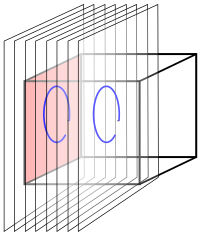
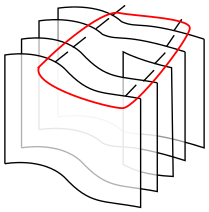
Electromagnetic Wave Simulator

I imagine readers are already overwhelmed by the formulas. Let us turn to the most intuitive thing: I used an AI to run a 2D‑time electromagnetic wave simulator: EM2T.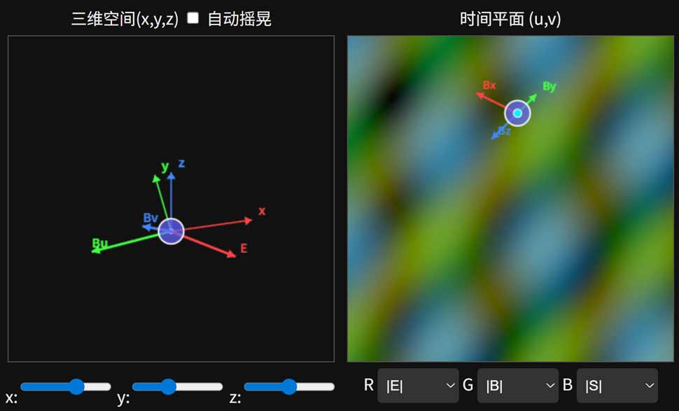

It has various preset electromagnetic waves, allowing intuitive visualisation of the field distributions in space and time. It is worth noting that the magnetic field is actually a $3\times2$ tensor, which can be viewed as two trivectors $\mathbf{B}_u$ and $\mathbf{B}_v$, or as three bivectors $\mathbf{B}_x$, $\mathbf{B}_y$, $\mathbf{B}_z$ on the time plane, giving a total of 6 degrees of freedom. The simulator displays both decompositions separately in 3D space and on the time plane.

Optional Reading: Waves and Quantum Mechanics

The Full Photon Puzzle

I wonder if readers have a question upon seeing these electromagnetic waves: since time is now 2D, why are we still using a wave vector — a one‑dimensional object — to describe the direction of propagation? Shouldn’t we use a bivector representing a plane? The monochromatic plane waves in the simulator still propagate in only one time direction, which gives the impression that these electromagnetic waves correspond to a kind of “half photon”: its world sheet is light‑like in one direction and time‑like in the other. Is there a “full photon” whose entire world sheet is light‑like in all directions? Unfortunately, I can only find superpositions of perpendicular half‑photons; the resulting combined wave appears to propagate over the 2D time plane, but I do not think this counts as a true full photon, and it is likely that full photons do not exist. Let us step away from the specific form of the electromagnetic field and discuss general waves.

2D Waves

We know that microscopic quantum theory is based on wave functions. A general wave has a phase factor that varies linearly with time and space; taking sine/cosine of the phase factor gives a periodic wave. To obtain a wave that propagates on a 2D plane like a full photon, we would need two phase factors, because if there is only one, the direction of its gradient (the direction of fastest change) on the time plane is the propagation direction, while the perpendicular direction is stationary — exactly the “half‑photon” mode we saw earlier. Suppose we have two phase factors; how do we combine them into a final wave? First, a wave must be periodic. To have 2D periodicity on a plane, the fundamental periodic region (i.e., the repeating unit) must be a parallelogram lattice. Such a lattice clearly breaks time‑rotation symmetry, so our full photon can no longer be a point‑like object; it may indeed only be a superposition of several half‑photons. To obtain an isotropic wave packet on the 2D time plane, we need at least two plane waves with different time directions. The interference pattern then has a parallelogrammic periodic region on the time plane, breaking continuous rotational symmetry and leaving only discrete lattice symmetry.

Quantisation Dilemma

Even if we accept that full photons can only be synthesised from half‑photons, that is not the most fatal problem. What truly puts 2D‑time quantum mechanics in trouble is the definition of the momentum operator. We know that the Fourier transform of a single‑particle position wave function gives the momentum wave function; the spatial frequency distribution determines the corresponding momentum components, and the momentum operator is the gradient operator $-i\hbar\nabla$, a first‑order derivative that acts on a scalar wave function to yield a vector. But in 2D time we have argued that momentum must be a bivector. It is impossible, within the framework of a scalar wave function, to find an operator that uses only first derivatives and produces a bivector — one would either have to use second derivatives or promote the scalar wave function to a vector or bivector field, but these structures are too complicated and amount to forcing a mathematical form, clearly indicating that something is wrong.

Noether’s theorem also supports this: it states that spacetime symmetry transformations yield corresponding conserved quantities. But regardless of the number of time dimensions, spacetime translations give a vector‑valued conserved momentum, not a bivector‑valued one. The conserved quantity from spacetime translation symmetry is always the vector momentum $P^a$, not a bivector. Although we could artificially define a two‑parameter spacetime translation, the resulting bivector would be non‑fundamental, just like a combination of half‑photons into a full photon. The bivector $P^{ab}$ we constructed earlier in non‑relativistic particle mechanics is actually a repackaging of the information contained in the 5D vector momentum; it is not a fundamental conserved quantity generated by an independent symmetry. Therefore, it is very likely that the canonical commutation relations in quantisation only hold for the vector momentum, and there is no independent bivector version of the momentum operator. This implies that directly extending scalar particle quantum mechanics to 2D time may face fundamental difficulties. Either we abandon the scalar wave function description and accept unnatural spin‑carrying fields as fundamental objects, or we redefine the rules of quantisation for 2D time. Fortunately, when studying only macroscopic phenomena, quantum mechanics is often not needed.

Game of Life?

So far we have discussed “real” physics in continuous time. Now let us look at a lighter topic: discrete‑time systems — cellular automata in 2D time. The Game of Life is the most famous cellular automaton. How can we generalise it to a 2D‑time version? Naturally, we want time to also be a discrete square grid, so the global state is described by integer lattice points $(x,y,u,v)$ in four dimensions. In the traditional Game of Life, the next state of a cell is determined by counting its 8 spatial neighbours. But in 2D time there is no preferred direction, so I took a different approach: can the number of spatial neighbours and the number of time neighbours constrain each other? For example, if both counts are within certain ranges, the middle cell must be dead; for other ranges it must be alive; for still others it does not matter. With the rule set, how do we simulate it? Since time no longer has a single direction, we cannot directly give a recurrence relation; we may have to find a global solution. I asked an AI to write a simulation program using the wave function collapse algorithm — CA2T. The illustration above shows a result of a small 2D‑time Game of Life with $5\times5$ space and $5\times5$ time. The left part shows spatial slices, the right shows time slices; grey indicates undetermined cells, and white dots represent live cells.

This Game of Life works as follows: First, a rule table is given, which is a $9\times9$ grid. The horizontal axis represents the number of time neighbours $n_t$ (08), and the vertical axis represents the number of spatial neighbours $n_s$ (08). Each cell of the rule table can be set to one of three states: must be dead (black), must be alive (white), or don’t care (grey). This rule table determines, for each cell, what state it must be in under a given spatiotemporal neighbourhood environment.

With the rules in place, how do we run it in 2D time? In the ordinary Game of Life, we only need to know the spatial state at the previous time step to evolve frame by frame into the future. But in 2D time, there is no one‑way past or future; time itself is a 2D plane, and we can no longer iterate along a single direction. Instead, we treat all cell states (0=dead, 1=alive) over the whole 4D grid $(x,y,u,v)$ as a whole and search for a global assignment that satisfies all neighbourhood rules simultaneously. We can use the Wave Function Collapse algorithm, which starts from a partially determined initial configuration and attempts to assign life/death to undetermined cells, backtracking whenever a contradiction is found, until all cells are determined (success) or a contradiction persists (failure). You can slide the mouse along the time axis to observe changes in the spatial state, or click on a spatial point to see its life/death trajectory over the entire time plane. During the solving process, the algorithm displays the neighbour counts of currently determined cells in real time, helping us confirm whether the cell states comply with the rules. In fact, for most rule tables, obtaining a global solution is quite difficult because we are working in 2D time plus 2D space — essentially a 4D spacetime. Each cell has two possible states, and the default grid is $5\times5$ in all dimensions, giving $2^{5^4}=2^{625}$ possible configurations. When backtracking, without special strategies, even if a solution exists, the search may take a very long time. I tried to optimise the backtracking mechanism generated by the AI, but it turned out that the optimisation made it harder to find solutions — a negative optimisation — so I stopped tinkering for now. If any reader is interested in this simulation, feel free to share your optimisation strategies. (Source code is on github)

2D Time Civilisation?

After exploring the various possibilities of 2D time, we cannot help but ask: what are the daily lives and subjective experiences of creatures living in 2D time like? I once discussed this topic with @kenzaki-ririka. The content is quite fanciful, so take it as entertainment without strict logic. Some parts are as follows:

• In this world, can 2D beings apply forces to objects to determine exactly how they move? For example, when kicking a ball, can they decide in which time direction it moves away from them and which direction brings it closer? I find it hard to imagine the actual operation, because the sequence of actions is also 2D.
• Cinema scheduling in a 2D‑time world: if the polygon‑shaped films cannot be densely tiled, it may affect the cinema’s profits. How do they know when to watch a movie? Should they give a boundary equation for the film’s showing time, but how is that coordinate system established? In other words, how do their celestial bodies rotate? The trouble with scheduling in 2D time is that you have to consider not only the area of time but also its shape. For example, when choosing songs at a KTV, you have to fit songs of different shapes into a chunk of time, which might lead to moments where no one is singing but everyone is just sitting there playing with their phones…
• Driving a car in 2D time: if there is an accident, the 2D person would not die. If the accident occurs at a point or inside a closed curve, one might even see fragments on the ground automatically fly up to repair the car and continue moving… Would the control system of a 2D car be different? Although the actions of the accelerator and steering wheel can also be 2D, the state at any given instant is deterministic. For example, the gear lever could move in different directions on the 2D time plane… How would road traffic differ? Would traffic lights at intersections alternate like a chessboard? But considering traffic flow and such, the lights probably would not be of the same size and shape, and one would also have to consider dense tiling. Moreover, roads might also have to be 2D — would intersections require 2D overpasses?
• Would day‑night cycles on their planet be checkerboard‑like? The rotation of a planet involves rigid‑body dynamics: the angular velocity also has $u$ and $v$ components. Through the action, one can derive the free rigid‑body equations of motion, and the orientation at each instant is determined by boundary conditions. Thus the rotation pattern can be very arbitrary, and the day‑night cycle might be extremely complicated…
• How do seasons work on their planet? Imagine a planet stably orbiting a central body. What does its world sheet look like? The orbital system is also determined by boundary conditions, with large freedom. I thought of some special cases: one possibility is that it moves in uniform circular motion in the $u$‑time parameter and is stationary in the $v$‑time parameter, but that does not capture the interesting structure of 2D time. Another possibility is to assume isotropy in the $u$ and $v$ directions, so that the orbital angle must have rotational symmetry on the time plane. This would imply a special instant — the centre of time‑plane rotation — which might be a distinctive feature of a 2D‑time galaxy?
• Analogous to our traffic light countdown, would a 2D intersection have a diagram showing the alternating pattern of the traffic lights, with a moving dot indicating the current time? Their video players might also show a diagram of the video’s shape below. Some short‑video platforms might automatically schedule videos via algorithms so that users can watch them with maximum efficiency. The parts that cannot be densely packed could be filled with advertisements…
• The articles, sentences, and words in a 2D language also have shapes. Therefore, when considering tiling issues, would writing be as brain‑twisting as composing parallel prose? If it becomes too difficult, one might have to fill the gaps with modal particles. The eight‑legged essays of the Ming and Qing dynasties in a 2D world might have strict requirements for such tiling? Perhaps the pronunciation of each character inherently has a shape, and there might even be something like “ideographic pronunciation”? Or maybe each character in some civilisations is pronounced as a standard hexagon or square?
• Dynasties in two dimensions might have complex shapes like countries in space, with revolutions or coups occurring along border lines?
• Since half‑photons are stationary in one time direction, could we capture a half‑photon flying through the air and press it into paper to write letters?
• If entropy determines the arrow of time, what happens when a 2D creature stirs coffee? If they only perceive the direction of entropy, they would see the milk mixing with the coffee but not yet fully mixed — entropy is increasing. However, macroscopic Newtonian mechanics would make them feel that the spoon is not completely in their control; other versions of themselves near the isoentropic line are also holding the spoon. Inertia connects the spoons in their hands, and even if they let go, the spoon would continue spinning in the coffee cup. In fact, the neurons/particles in their brains are like this spoon, jointly carrying out thought processes — they are all part of the memory of the same 2D creature at different time directions. Therefore, I think the way 2D creatures experience time cannot be solely through the direction of entropy increase. Entropy may influence their consciousness, but not as absolutely as for us. On the time plane, there are extrema of entropy; consciousness might get trapped inside them. But could they store some negative entropy, travel against the total entropy gradient for a while, and reach another region with stable entropy increase, somewhat like quantum tunnelling through an entropy barrier?
• If I break a cup at just one instant, what shape does the broken cup have in time? When a 2D person gets sick and takes medicine, what is the function of the drug concentration on the time plane? If we want the patient to have both the encapsulated and the diffused states simultaneously over an infinite range of time, the boundary between the two states would be a one‑dimensional line. That means taking the medicine is not a point‑like event; the patient would have to swallow the capsule along an infinite time line? But that sounds like a time “cylinder”, equivalent to squeezing one time dimension out of our world. If there is no change along that direction, we might not even notice its existence. In other words, if the capsule dissolves along a line, is that equivalent to the normal dissolution of a capsule in our one‑dimensional time?

Sci‑Fi Setting: Time Divers

The last question leads us to wonder why we perceive the world as having only one dimension of time. One idea is that we actually live in a complete 3+2 dimensional universe, but our local spacetime region is extremely flat in the $v$‑time direction — so flat that almost no events change along the $v$ direction. Physically, this means that the world sheets of all matter in this region have near‑zero curvature in the $v$ direction, like a tightly stretched membrane, completely stationary along that direction. The natives of the 2D time world, while exploring their universe, discover this anomalous region. To them, this “time frozen land” is fragile: any foreign world sheet with variations along the $v$ direction that intersects it will create ripples on this flat surface — like a stone thrown into still water. Once these ripples spread, they could completely alter the physical structure of the region. For protection — and perhaps out of reverence — they developed a special technology: compress the variation of their own world sheet’s $v$ component to nearly zero, i.e., “freeze” themselves in one time direction, moving only along our $u$‑time direction. In this way, they can quietly enter our time slice without disturbing the flatness in the $v$ direction. They do not come by walking; they “live” into it as 2D time flows — they call themselves Time Divers. After diving in, they lose the freedom to walk freely on the $u$‑$v$ plane and are locked onto the one‑way $u$‑axis, experiencing time frame by frame just like us. But they discover Earth civilisation, a wonderful species that spontaneously emerged on this time frozen land. Out of protection, and also out of some indescribable sentiment, these divers choose to stay. They abandon their 2D‑time homeland and live among us entirely in the one‑dimensional‑time lifestyle…

Crazy idea: Spacetime Swap?

I wonder if readers have ever questioned why one dimension is perceived as time, simply because its coefficient in the metric is negative? Why not still treat this coordinate as space? From the spacetime metric, time and space do exhibit a kind of duality — 2D time + 3D space is in some sense equivalent to 2D space + 3D time. 3D time would be even more complex, so we can step down and consider the case of 2D space + 2D time: could there be two forms of life coexisting, each treating the other’s time as space? That is, a creature A’s world sheet appears timelike to itself but spacelike to another creature B? What kind of interactions would they have? Physicists have hypothesised the existence of superluminal “tachyons” in our spacetime, but their trajectories are one‑dimensional, not the type of spacetime‑swapped matter we are looking for. Could there exist, in the same universe as us, a kind of matter whose world‑volume ( 3D manifold) lies in our space, while what we call time is for it a spatial direction?