4D Space (XII): Unknotting Spherical Knots
# This article is a sequel to 《Four-Dimensional Space (X): Knots and Links》. This content requires high spatial imagination and may be difficult to understand in some places, but the entire article contains no formulas and only involves geometry, not algebra, making it suitable for challenging spatial imagination!
# I’ve discovered that not only me, but everyone online is mixing up “knot” terminology, so I won’t bother to correct it either.
In the previous article of this series, we learned about knotting phenomena of two-dimensional surfaces in four-dimensional space and various types of holes, links, etc. The introduction to two-dimensional surface knots wasn’t actually very detailed last time - we only gave some non-trivial tubular knots as examples. Today we want to analyze knots from another perspective. The main content of this article comes from this YouTube video and this paper, which introduces how to construct knots homeomorphic to spheres by rotating trefoil knots (i.e., knots that can be restored to spheres if self-intersections are allowed), and proves that some are truly impossible to unknot while others can be unknotted into spheres through certain steps. Let’s try to unknot some knots in high-dimensional space!
Revolution of a Knot
Actually, we already discussed using rotation to create non-trivial knots in the previous article. Let’s review: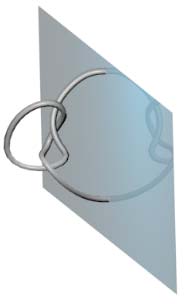
A semicircle rotated once around can yield a sphere. A semicircle with a knot tied in it, when rotated once around in four-dimensional space, can yield a type of knotted sphere. Note that rotation in three-dimensional space would result in self-intersecting surfaces. That article also mentioned that if we call rotating knots “revolution,” then knots can also “rotate” during the revolution process, yielding some more complex knots with additional “spin.” This article is about doing exactly such a thing:
Rotational spherical knots with 360-degree spin can be unknotted!
Intersections on 3D Knot Projections
Following our traditional practice, let’s first study knots in three-dimensional space. For example, here’s a trefoil knot (the simplest non-trivial knot). How do we describe it to two-dimensional beings? The topological essence of a trefoil knot is a circle (actually, all knots in three-dimensional space are!). We find a point O and directly cut the circle open (but note that topology doesn’t allow directly cutting objects, so we must be able to glue the two ends back together at any time). Starting from point O, we will pass through three intersection points in the projection. To preserve as much information as possible, we note which intersection points correspond to which, and record whether we pass over or under each intersection point (if we go over, we write the letter above the line; if we go under, we write it below), finally obtaining a line like the one on the right in the diagram below:
Below I give a line - can you restore the original knot projection diagram?
Think about it first…
The restoration method is simple. We draw a line and mark the corresponding intersection points on it. When we encounter a previously marked point, we thread the line through that intersection point and continue repeating the above process until we complete the circuit. We discover that except for the first time we encounter a previously marked point, when we can choose between threading from the left or right (two topologically non-equivalent drawing methods), all other connection methods are fixed, as proven by Alexander. Note that there are many projection angles; the above discussion is all conducted on any specific projection.
Now I tell you that the knot above can be unknotted into a circle. You’re certainly not surprised because this is obvious, but now you need to convince our friends from the two-dimensional world. You can explain the legal deformation moves for knot projections (Reidemeister moves) to them, thereby rigorously unknotting the knot above step by step. But when they see these complex self-intersections in two-dimensional space, they feel overwhelmed (their vision is one-dimensional). What should we do? We can let them understand only what happens to those intersection points on the circle, without worrying about the rest. The specific method is to correspond each legal move to some changes in intersection points on the circle unfolding diagram! (Yes! We’ll also use the upgraded version of this method to handle spherical knots later)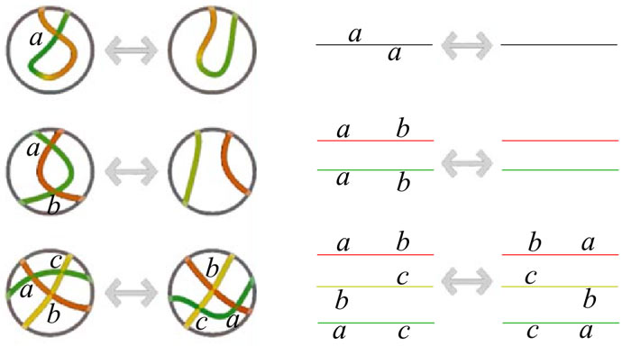
Note that this method can only prove that two knots can become equivalent through legal moves, but cannot prove that two knots are not equivalent. Fortunately, we’ll only be unfolding a spherical knot later to prove it’s equivalent to a sphere.
Perhaps you find these letters on the line too abstract. Then we can use the time axis as another axis, so we can draw the process of intersection point changes during movement. Note that points moving create lines, so the original intersection points become trajectories. We now use red to represent intersection point trajectories passing from above, and blue for those passing from below. Note that the third type of legal move involves three lines, so there are three parallel time trajectory diagrams:
Notice that all three types of moves have a “bad” critical position in the middle (for example, in the first diagram, the projection has a cusp where two intersection points cancel out). Generally, we avoid these in knot projections, but during movement, these states are unavoidable.
Perhaps you’ve already noticed that if we view the time axis as space, these diagrams are intersection traces of some two-dimensional knots in four-dimensional space. But before formally discussing intersection traces of two-dimensional knots, let’s first visualize our protagonist - the rotating spherical knot.
New Four-Dimensional Graphics Visualization Method
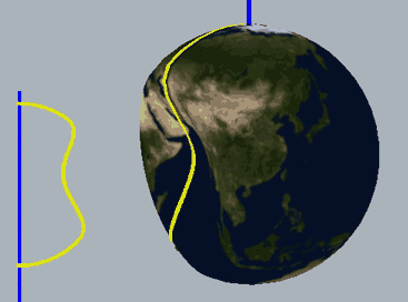
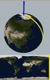
We need to first understand what a “rotational spherical knot with 360-degree spin” is before we can talk about unknotting it. We’re already dealing with abstract four-dimensional space, then adding revolution, spin, and deformation - we face what seems like an impossible task. But by breaking this task down piece by piece, we’ll discover it’s not too difficult. First, I want to introduce a new method for visualizing four-dimensional graphics - it’s a type of cross-section method. But unlike previous methods of having four-dimensional objects pass through three-dimensional planes from one direction, this uses a rotational cross-section method more suitable for rotational bodies: if a figure is a perfect rotational body, its cross-sections at different angles are the same, but for non-rotational bodies, cross-sections taken from different angles won’t necessarily be the same. So we fix the rotational plane and observe and describe this four-dimensional object by observing and describing changes in the figures on the rotational plane through one complete rotation. This method is actually equivalent to cross-section method along the rotational direction in polar coordinates. To better understand, let’s only consider the cross-section line animation of a two-dimensional sphere in three-dimensional space: we unfold the sphere like a world map into a rectangle, and the rotational cross-sections on the sphere (some great semicircles) also become ordinary cross-sections in the longitudinal direction on the world map. If this sphere has one side that’s flattened, our rotational cross-section animation can accurately reflect these deformations.
|
|
|
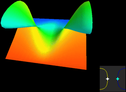
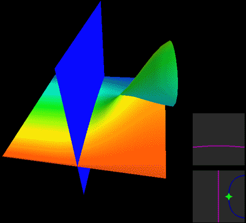
We know that a hypersphere can be obtained by rotating a two-dimensional hemisphere around a plane (this should be obvious to readers who can see this far). For example, everyone should be able to understand that the rotational cross-section animation below describes a hypersphere with one side concave and one side convex:
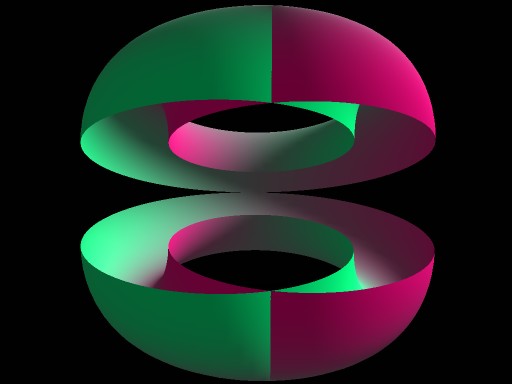
Below, we place a two-dimensional sphere in four-dimensional space and use this method to look at spheres, non-self-rotating rotational spherical knots, and spherical knots with one full spin. Note that the first two are rotationally symmetric figures, so their cross-sections don’t change: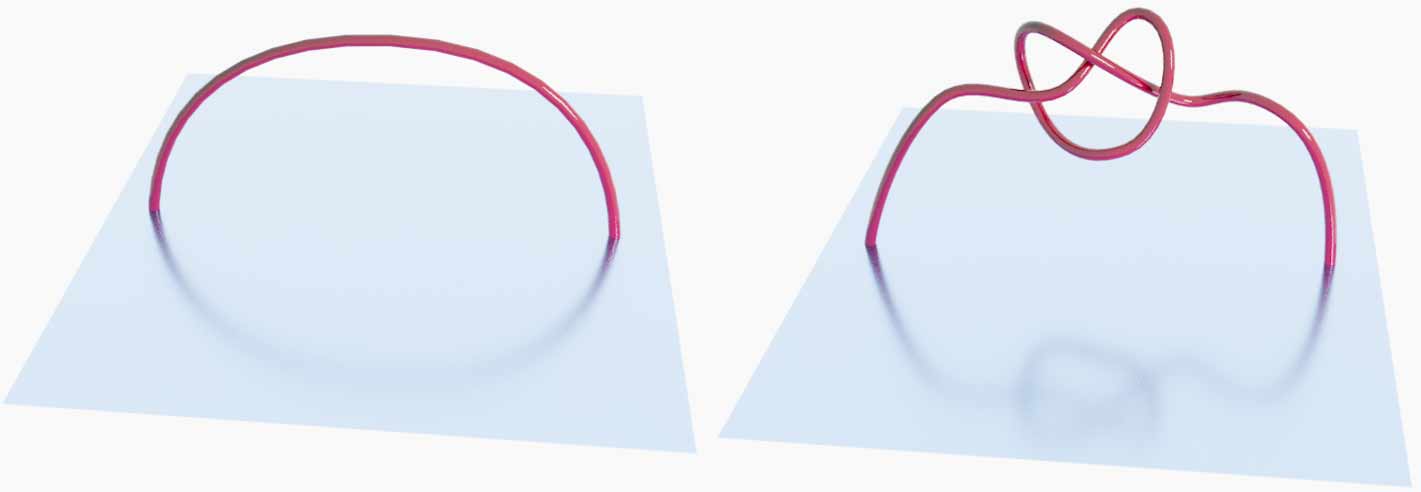
What we want to prove is that this constantly self-rotating revolutionary cross-section animation can be continuously transformed into a sphere without tearing!
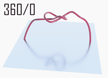
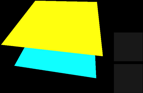
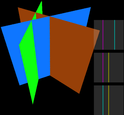
The two types of spherical knots projected directly into three-dimensional space look like: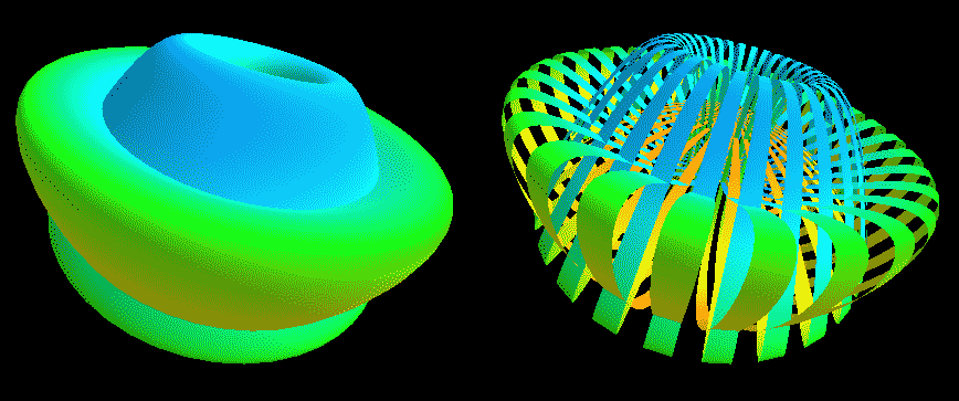
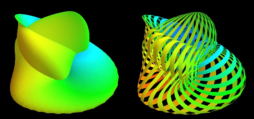
The right diagrams in these two figures hollow out the surface into strips of rotational cross-section slices to observe the interior of the surface, where one dimension is compressed in the rotational cross-section slices on the projection, so we use coloring to represent this direction. Therefore, you’ll see that each slice strip has self-intersections in the projection. Note that the relationship between revolution and spin here is somewhat different from the Earth-Sun system (not considering the simple system of seasons). In the Earth-Sun system, both revolution and spin planes are absolutely parallel, while in this knot, the spin and revolution planes differ by 90 degrees, in a half-parallel, half-perpendicular relationship. If we extract a single point and draw its trajectory in three-dimensional space, we can see that the Earth-Sun system trajectory has serious self-intersections, but the self-rotating knot doesn’t.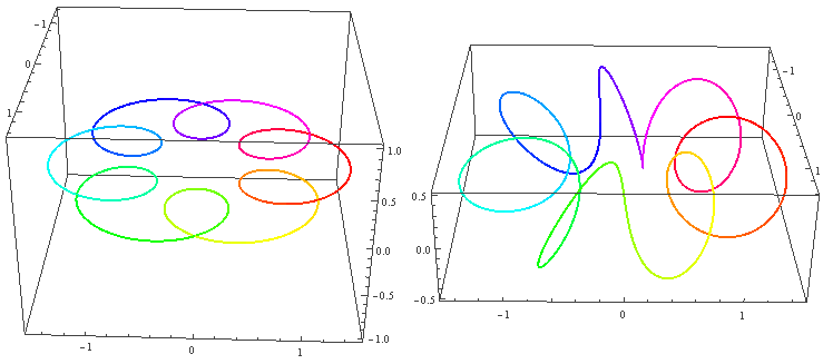
If your spatial imagination is good, you should be able to imagine the cross-section animation of a non-self-rotating rotational spherical knot along the symmetry axis (ordinary translation) - it’s the rotational body of an ordinary knot’s cross-section animation (there’s a universal conclusion: the rotational body of a cross-section animation is the cross-section animation of a rotational body!). The core of knots is the intersection points of projections, so we must understand how this surface self-intersects. But the structure of the second one seems very difficult to understand - it’s almost impossible to imagine the overlap pattern of projections with revolution plus spin out of thin air. So we urgently need a new dimensionality reduction method. Fortunately, we’re studying topology, and our research object is just a sphere. Rather than studying intersection traces of projections on a spherical knot in four-dimensional space, we might as well unfold the sphere like a world map and focus all our energy on two-dimensional space, just like showing string loops to friends from the two-dimensional world, to see what these intersection traces look like when unfolded.
Intersection Lines on Maps
Let’s first look at the overlapping lines of projections of non-self-rotating rotational knots. Remember the circle unfolding diagram of the trefoil knot projection? Since the projection of a non-self-rotating rotational knot is a perfect rotational body, the trefoil knot always remains unchanged, and these intersection points also remain unchanged during rotation. So we’ll get some circular intersection lines, which become latitude lines when unfolded. Note the annotation of whether the surface passes through the intersection line from above or below when projections overlap - here we distinguish with red and blue colors.
Let’s look at a tubular spherical knot mentioned in the previous article. We’ll try to draw the intersection traces on the unfolding diagram of this projection.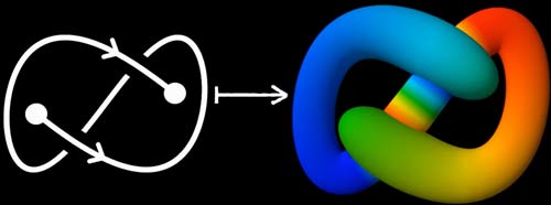
Although this tube doesn’t have rotational symmetry, we find it can be divided section by section along latitude lines (black lines in the diagram below), so we can directly find correspondences on the world map and start drawing. (In topology, as long as we can establish mapping relationships, the specific positioning doesn’t matter) First, starting from the green north pole, the left and right sides are passed through by the tube from the middle, forming two intersection circles. We mark the intersection circles as a and b, noting that intersection trace b has green higher than blue (red has the highest altitude, blue the lowest), so we mark it with a red line. Intersection trace a has green lower than red, so we mark it with a blue line. Then we pass through yellow and red, through the cyan south pole, forming two intersection circles c and d. Note that unlike the intersection circles obtained by being passed through when we first started, here we actively pass through the south pole, so the two intersection circles are latitude circles, which will be cut open and become straight lines when drawing the world map. Then we leave from circle d, with color rapidly rising from blue to red, arriving at the previous a, b intersection circles, which are now also latitude circles that can be cut open. After passing circle b, we reach near the south pole, where there are also the c, d intersection circles.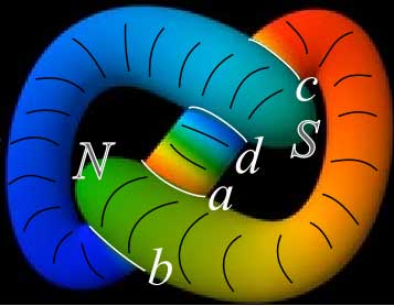
If you understand, you should be able to draw such a map (note that the world map direction is north up, south down)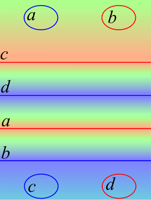
Self-Rotating Trefoil Knot
How do intersection traces change if knots undergo spin during revolution? Obviously, the lines on the world map will become complex. Note that when knots rotate, their projections must be performing the 3 types of legal moves for one-dimensional knots, so we need to reconstruct the intersection lines on the world map through these legal moves. This is like taking the longitude direction as the time axis and upgrading the one-dimensional unfolding diagram of self-rotating knots to two dimensions by adding time.
Let’s first draw the spin projection process of the one-dimensional trefoil knot following the previous rotational cross-section animation. We can draw only some key frames like animation production, but here each frame is a legal move. Drawing these projections involves quite a bit of work and seems somewhat tedious.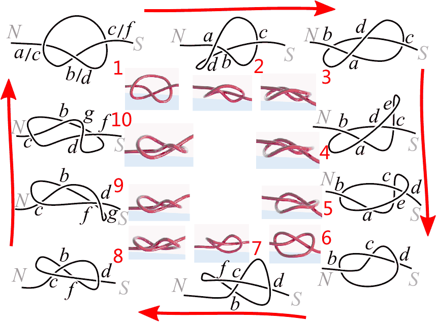
We see that after the trefoil knot rotates once, the numbering of intersection points changes, but this doesn’t matter. Starting from projection 1 in the upper left corner, let’s set the intersection points as a, b, c respectively. Projection 2 inserts a type 1 legal move between a and b, adding an intersection point d. Note that at the moment intersection point d is generated, the projection will produce a “bad” cusp. Projection 3 uses a type 3 legal move on the triangular region a, b, d to “flip” its position, where at some moment during the transition from projection 2 to projection 3, three lines will coincide at one point. Drawing the above projections, we get the diagram below. Note that we need to mark the positions of triple points and cusp points in the projection.
In the diagram, the vertical direction is the meridian direction of the sphere, and the horizontal direction is the latitude or time axis (rotation direction). Therefore, vertical dashed lines represent the unfolding diagram of the trefoil knot at a certain moment. For example, moment 1 corresponds to projection 1, whose intersection points can be read from the dashed line from north to south as a b c a b c. Moment 2 is a b c a d d b c. Moment 3 is b a c d a b d c. You can walk through projections 1, 2, 3 once to verify whether the colors and order of these letters are correct.
Let’s continue rotating from projection 3 to projection 6. Actually, the intermediate process is very similar to before. Projections 3 to 4 use a type 1 legal move to generate intersection point e, projections 4 to 5 use a type 3 legal move to flip triangle cde, projections 5 to 6 use a type 2 legal move to eliminate intersection points a and e, where at the moment the two points are eliminated, two curves in the projection produce a “bad” tangent point. We can easily continue drawing this part of the map:
We can now figure out the pattern of these three types of legal moves. Actually, they repeatedly use this rotated 90-degree version of the diagram from the previous section. Looking at it now, doesn’t it feel different?
Drawing all of 1-10, we can get the complete world map:
Note that the connection between the east and west sides of the world map is consistent with the letters on both sides of the slash in projection 1, and these red and blue curves are actually drawn on the sphere.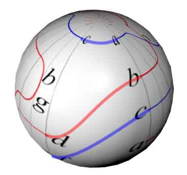
Note that we just viewed this diagram from the perspective of the time axis. If we look at it from the perspective of four-dimensional space, the cusps generated in type 1 legal moves correspond to branch points on two-dimensional surfaces, the triple points generated in type 3 legal moves correspond to three two-dimensional planes intersecting pairwise with a common triple intersection point. Type 2 legal moves don’t actually generate singular points - we can see from the map that there’s no singularity on the intersection lines of type 2 legal moves; it’s just that our chosen coordinates aren’t good (somewhat like the singularity on the event horizon of a black hole).
Four-dimensional space is isotropic, so the “time axis” direction isn’t special. Therefore, we can deform and simplify the world map above. Note that from now on we no longer mark projection intersection points (they only have meaning after choosing a time axis), but mark corresponding points in projections through triple intersection points (numbered).
Seven Types of Legal Roseman Moves
We can now draw these intersection lines, but when we change the viewing angle or stretch two-dimensional knots, the overlap situation of these projection intersection lines will certainly change. As mentioned before, similar to the 3 types of Reidemeister moves for one-dimensional knots, mathematician Roseman summarized 7 types of legal moves for two-dimensional knots, so we need to study the patterns of projection intersection line changes corresponding to these 7 types of legal moves.
Let’s get straight to the diagrams:
Roseman move 1 has branch points in the projection, which might not be very intuitive. The previous article mentioned using cross-section method to understand this Roseman move.
Roseman move 2 has branch points in the projection, also understood through cross-section method.
Roseman move 3 is the easiest to understand because the fourth dimensional color of the two surfaces is constant - we only need to focus on the trace changes in the three-dimensional projection.
In Roseman move 4, the fourth dimensional color of the two surfaces is also constant - we only need to look at the traces in three dimensions, which is also easy to understand.
In Roseman move 5, all surfaces have constant fourth dimensional color.
In Roseman move 6, although one surface has branch points, the other plane is blue, indicating it’s at the very back in the fourth dimension. The movement of the surface with branch points in front naturally won’t affect the plane in back.
Although Roseman move 7 involves four surfaces, all surfaces have constant fourth dimensional color.
Using Roseman Moves to Unknot It!
Warm-up
Let’s not rush. Before formally unknotting rotational spherical knots, let’s solve some other simple problems first (or you can try unknotting rotational spherical knots independently):
- The previous article drew projection diagrams of flat tori. Let’s use legal Roseman moves for intersection lines to prove that this projection can be stretched into a general tire torus in four-dimensional space.
The torus unfolding diagram is a rectangle. This flat torus’s three-dimensional projection has two double intersection lines parallel to meridians and four branch points. After unfolding, it looks like the diagram:
According to Roseman move 2, two branch points can merge when their directions are consistent, giving us two circles. Finally, we find these two circles can be removed using Roseman move 3. At this point, all intersection traces in the three-dimensional projection disappear, meaning this projection becomes a tire torus without any self-intersections.
- Klein bottles cannot be embedded in three-dimensional space unless self-intersections are allowed. Common self-intersecting models include not only the bottle shape that passes through itself but also the type shown below. Let’s use legal Roseman moves for Klein bottle intersection lines to prove the two are topologically equivalent. (Actually, we also proved they’re isotopic in four-dimensional space, meaning one can be continuously transformed into the other)
This projection is very similar to the flat torus, except it has only one double intersection line and two branch points - half as many as the flat torus. We directly use Roseman move 2 to merge these two branch points, obtaining two closed circles, one of which is a normal small circle (red), while the other circle spans the entire meridian and cannot be shrunk (blue). Red corresponds to intersection traces on the Klein bottle’s belly, blue corresponds to intersection traces on the Klein bottle’s neck.
- The previous article mentioned that even with fixed tube endpoints, tubular knots passing through themselves can be unknotted. Directly imagining the unknotting process is somewhat difficult, so let’s also use legal Roseman moves for intersection lines to prove it.
First, we observe that there are two intersection traces on the tubular knot. We mark them as A and B from left to right. Starting from the left tube mouth, passing in and out of itself, we get penetrating intersection traces A and B, then coming around to be passed through by itself, we get two non-penetrating circular intersection traces. We first use legal Roseman move 2 to split intersection trace B into a pair of branch points, then use Roseman move 4 on intersection traces A and B to connect the two intersection traces. After organizing, we find the current intersection trace is a circle with a pair of branch points, consistent with Roseman move 1, which can contract and disappear.
Now we’re going to unknot spherical knots. I strongly recommend trying it yourself first - the unknotting steps aren’t unique, so what follows is just my reference.
Unknotting Spherical Knots
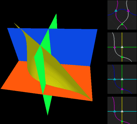
Based on experience from the three problems above, let’s first try directly merging branch points. Observing, we find that the branch points marked 1 and 4 on both sides can meet, and the branch points marked 2 and 3 on both sides can also meet. Remember this is an unfolding diagram of a sphere, so we can cross over to the other side like crossing the “International Date Line.”
We first use Roseman move 2 to merge the branch points marked 1 and 4 on both sides.
Then merge the branch points marked 2 and 3 on both sides. Note how the intersection lines cross the “International Date Line.”
The sphere’s unfolding diagram indeed looks inconvenient due to the “International Date Line.” We might as well directly connect the corresponding sides, transforming it into something like a stereographic projection map. As long as intersection lines don’t pass through the pole, the map has no edges at all. Note that choosing to go around from above or below relates to the position chosen for the north pole in stereographic projection.
After some organization, we can get 4 “figure-eight” shaped intersection lines in the diagram below. They intersect end-to-end in a ring formation, meaning all intersection traces now have only double intersection lines and triple intersection points.
Before we continue looking for usable Roseman moves, let’s first clarify that this diagram is an unfolding diagram where points on intersection lines have mutual correspondence relationships. Let’s observe what properties a meaningful intersection line unfolding diagram has, so we don’t mistakenly use Roseman moves without knowing it.
- First, we’ve marked 4 triple intersection points with numbers. Although the 4 “figure-eight” shapes have 12 intersection points total, positions with the same number correspond to the same point in three-dimensional projection space when the sphere is folded up. We can also observe that these triple points with the same number must have one that’s all red lines intersecting, one that’s all blue lines intersecting, and one that’s one red and one blue intersecting, because they must correspond to the frontmost surface, rearmost surface, and middle surface in the fourth dimension.
- When we leave a triple point and walk along a line, this line is the intersection line of two surfaces, so there will be paired red and blue intersection lines on the unfolding diagram. If we arrive at the next triple point, the two intersection lines on the unfolding diagram will also arrive at this point. For example, for the red figure-eight below, it might pair with the blue figure-eight above or to the right, but which one exactly? Walking around the red figure-eight below, the triple points passed are 2-1-3-2-4-3. Starting from 2 on the upper figure-eight, we can also get 2-1-3-2-4-3, while the right figure-eight can’t match 2-1-3-2-4-3 in any direction, so the upper and lower figure-eights pair. Similarly, we can verify that the left and right figure-eights pair.

- Although we’ve eliminated branch points now, from the previous diagram with branch points, we can see that branch points are special points where paired red and blue intersection lines emerge. Branch points correspond to themselves. Here’s a wild idea: branch points are somewhat like the time reversal machines in the movie “Tenet” - red lines become blue after passing through, and all passed triple points are traversed in reverse order like time flowing backward.
Since no branch points are involved, we can try using Roseman moves 4, 5, 7 to solve. Roseman move 4 can reconnect two line segments of the same color, but we must simultaneously change both paired red and blue ones. At first glance, it’s easy to implement Roseman move 4, but there aren’t many moves that simultaneously satisfy both conditions. For example, if you want to use Roseman move 4 on red 1-4 and 3-4 along the black arrow direction, you must also use Roseman move 4 on blue 1-4 and 3-4, but unfortunately there are other intersection lines between them, preventing the move. Here we also need to note that there are two blue 1-4 line segments on the right figure-eight - how do we know which is the paired line segment? We notice that one line segment continues from 1 to 3, while the other continues from 1 to 2, and our chosen red line segment continues from 1 to 3, so the former pairs with the chosen red line segment.
Are there choices that allow Roseman move 4? Yes, I’ve marked some choices here (there should actually be more):
Before deciding which choice to make, let’s look at Roseman moves 5 and 7. Roseman move 5 either finds three pairs of parallel lines, letting them intersect to get three “bigon” regions, or finds three corresponding “bigon” regions and unknots them into three pairs of parallel lines. The connection of two figure-eights creates exactly one “bigon” region, but unfortunately, these “bigon” regions don’t correspond to other “bigon” regions, so no “bigon” can be unknotted using Roseman move 5, as shown below. Can we choose three parallel lines and use Roseman move 5 to make them intersect, creating three “bigon” regions? This would increase the number of intersection points, going against unknotting, so we abandon Roseman move 5.
Let’s look at Roseman move 7. Roseman move 7 is also very distinctive - it needs to find four triangular structures with correspondence relationships. We find that after drawing the corresponding sides of the shaded triangle 134 in the upper left corner, the corresponding sides and triple point 2 can all form triangles, so this conforms to Roseman move 7.
Now we have Roseman moves 4 and 7 before us. Let’s look at Roseman move 4 first.
We first do moves A and B, finding that there doesn’t seem to be much progress.
If we switch to move C, we can connect the two figure-eights together, and we find that this produces three corresponding bigons that can use Roseman move 5.
Let’s continue with Roseman move 5. We find that the figure after the move has become very simple - it’s two knotted circles. To unknot them, we use Roseman move 4 to split the circles in two, then find we can use Roseman move 5 again. Finally, we get four separate circles, which we eliminate with Roseman move 3, removing all intersection lines. At this point, we’ve completely unknotted the rotational spherical knot.
Alternative Solution
If we use the previously mentioned Roseman move 7, it would link the 4 figure-eights together without simplifying the problem. So is the method above the only way to unknot rotational spherical knots? Of course not - that’s just one approach I figured out personally. Actually, this YouTube video shows steps that directly use Roseman moves 4 and 5, then use Roseman move 1 to eliminate branch points, while this article eliminated all branch points in the first step, requiring more steps than the YouTube video.


Note that since we’re on a sphere, that large circle with branch points can separate from the inner circle by passing through the north pole, so this is a typical case of Roseman move 1, which can directly eliminate all intersection traces.
Well, this article ends here. As for how to prove that knots rotated twice cannot be unknotted, that’s the next topic. Although all the topological deformations described in this article occur in four-dimensional Euclidean geometric space, some people might not like topology. If possible in the future, I might start a new series about topology.