4D Computer Graphics: Modeling

4D Computer Graphics: Rendering discussed how to render 4D geometries but hasn’t mentioned where the data for these 4D geometries comes from. This article explores and summarizes common 4D geometry data generation algorithms.

Feature Content

• pyramid/Extrusion/Direct Product Generation
• Parametric Surface Generation
• Regular Polytope Generation
• Orientation Processing of Cell Complexes
• Tetrahedral Decomposition Problems

Brief Review

As the fundamental knowledge for this article, let’s first review the cell complexes introduced in the previous article: except for the vertex coordinates, which need to be described separately, we describe the boundaries of other higher-dimensional faces by the indices of the edges that make up those faces. For example:

1. A point:
   Vertex: {()₀}
2. A line segment:
   Vertex: {(-1)₀,(1)₁}
   Edge: {(0,1)₀}
3. A square:
   Vertex: {(-1,-1)₀,(-1,1)₁,(1,1)₂,(1,-1)₃}
   Edge: {(0,1)₀,(1,2)₁,(2,3)₂,(3,0)₃}
   Face: {(0,1,2,3)₀}
4. A square pyramid:
   Vertex: {(-1,-1,0)₀,(-1,1,0)₁,(1,1,0)₂,(1,-1,0)₃,(0,0,1)₄}
   Edge: {(0,1)₀,(1,2)₁,(2,3)₂,(3,0)₃,(4,0)₄,(4,1)₅,(4,2)₆,(4,3)₇}
   Face: {(0,1,2,3)₀,(0,4,5)₁,(1,5,6)₂,(2,6,7)₃,(3,4,7)₄}
   Cell: {(0,1,2,3,4)₀}
5. A cube:
   Vertex：{(1,1,1)₀,(1,1,-1)₁,(1,-1,1)₂,(1,-1,-1)₃,(-1,1,1)₄,(-1,1,-1)₅,(-1,-1,1)₆,(-1,-1,-1)₇}
   Edge：{(0,1)₀,(1,3)₁,(2,3)₂,(0,2)₃, (4,5)₄,(5,7)₅,(6,7)₆,(4,6)₇, (0,4)₈,(1,5)₉,(2,6)₁₀,(3,7)₁₁}
   Face：{(0,4,8,9)₀,(1,5,9,11)₁,(2,6,10,11)₂,(3,7,8,10)₃,(0,1,2,3)₄,(4,5,6,7)₅}
   Cell：{(0,1,2,3,4,5)₀}
6. The same for 4D geometries, but with more than one cellular data. e.g. a regular 5-cell:
   Vertex：{$(1/\sqrt{10},1/\sqrt{6},1/\sqrt{3},1)$₀,$(1/\sqrt{10},1/\sqrt{6},1/\sqrt{3},-1)$₁,$(1/\sqrt{10},1/\sqrt{6},-2/\sqrt{3},0)$₂,$(1/\sqrt{10},-\sqrt{3/2},0,0)$₃,$(-2\sqrt{2/5},0,0,0)$₄}
   Edge：{(0,1)₀,(0,2)₁,(0,3)₂,(0,4)₃,(1,2)₄,(1,3)₅,(1,4)₆,(2,3)₇, (2,4)₈,(3,4)₉}
   Face：{(0,1,4)₀,(0,2,5)₁,(1,2,7)₂,(4,5,7)₃,(0,3,6)₄,(1,3,8)₅,(4,6,8)₆,(5,6,9)₇,(2,3,9)₈,(7,8,9)₉}
   Cell：{(0,1,2,3)₀,(0,4,5,6)₁,(1,4,7,8)₂,(2,5,8,9)₃,(3,6,7,9)₄}

Note that the 5-cell (pentachoron) itself is also a 4D cell complex.The 4th dimiension of cell complexes could be introduced, but for 4D geometric rendering, knowing the 3D cells is sufficient. The 4D cell structure is generally not needed, so it has not been included above.

Common 4D Mesh Generation Algorithms

Simple shapes can be manually written out, but for more complex shapes, generation algorithms are necessary. Common generation algorithms include pyramidal construction, extrusion, direct product, etc. In fact, many 3D algorithms can also be extended to 4D, such as convex hull algorithms, implicit function surface modeling, mesh subdivision algorithms, Boolean operations, etc. Discussing these topics thoroughly could easily turn into a book as thick as a brick, and we do not have the resources to implement all of them. Here, we will cover some simple and practical generation algorithms, starting with the most basic pyramidal construction.

Pyramidal Construction

For a flat cell complex C, we can perform the pyramidal construction by finding a point outside the hyperplane where it resides, and this point will serve as the apex of the pyramid. The pyramidal construction can be recursively described: given a point P, the pyramidal construction of an n-dimensional cell is a new (n+1)-dimensional cell formed by adding the new vertex P. The boundary of this new cell consists of the original n-dimensional cell and the pyramidal construction of all its (n-1)-dimensional boundaries. Since a point has no boundaries, its pyramidal construction is special: it’s just a line segment with the point and P as the endpoints.

The usual programming algorithm is closer to a bottom-up approach: given point P, add it to the vertex list of the cell complex; then, connect it to all the vertices in the original complex to form new edges and add them to the edge list; next, the original edges, along with the new edges formed by connecting the endpoints of each edge to P, will form new triangular faces, which are then added to the face list; finally, the original faces, along with the new faces formed by connecting the boundaries of each face to P, will form new cells, and these will be added to the cell list…

Extrusion

Unlike coneification, which connects each element to a fixed point, extrusion involves translating the entire complex and then connecting each element from the original and copied complex to form a cylindrical shape. For a flat cell complex C, extrusion is performed by giving a vector not parallel to the hyperplane it resides in. Given vector V, the first step is to copy the entire cell complex and translate it along the vector. During this process, the vertices and each n-dimensional cell are duplicated, forming the “top” and “bottom” faces of the cylinder. Then, to generate the lateral surfaces: the lateral surface of each n-dimensional cell is made up of these boundaries: one from the n-dimensional cell on the bottom face, one from the corresponding n-dimensional cell copied to the top face, and one from the boundary of the original n-dimensional cell. Similarly, for points, their lateral surface is simply a line segment between the point on the bottom and the point on the top.

Direct Product

Understanding the direct product is not as easy as extrusion and coneification due to the lack of an intuitive 3D analogy. The direct product is more easily understood algebraically: it is a form of multiplication. For instance, it satisfies properties such as distributivity, commutativity, and associativity, and the direct product of an n-dimensional shape and an m-dimensional shape results in an n+m dimensional shape. I previously mentioned the geometric scene involving direct products in Tesserxel II: Scene Interaction under the “Direct Product Shape” section. The direct product shape $A \times B$ has two boundaries: one is the boundary of $A$ with the direct product of $B$, and the other is the boundary of $B$ with the direct product of $A$. The formula is: $$\partial(A \times B) = \partial A \times B + A \times \partial B$$Using this formula, we can construct direct product shapes from low dimensions to high dimensions. For example, for the direct product of two 2D shapes, we first duplicate shape A by the number of vertices in shape B, with the x and y coordinates of each duplicated shape remaining the same, and the z and w coordinates set to the x and y coordinates of the vertices of shape B. Now we have all the vertices of the direct product shape. This operation is equivalent to completing the direct product of all the n-dimensional cells of shape A with the 0-dimensional cells of shape B. Moving on, for $m=1$, we construct the direct product of each n-dimensional cell of A with each 1-dimensional cell of B, then for $m=2$, we construct the direct product of each n-dimensional cell of A with each 2D face of B… Note that when adding the $n+m$-dimensional cells to the cell list, a separate direct product index table must be maintained, with the key being the indices of the original n-dimensional and m-dimensional cells, and the value being the identifier of the $n+m$-dimensional cell, which will be used later to construct the boundaries of higher-dimensional cells’ direct products.

Revolution and Parametric Surfaces

A solid of revolution can topologically be viewed as the direct product of a section and a circle. For example, the topology of a torus in 3D space is equivalent to the direct product of two circles, and although the result should theoretically be a 4D shape (Clifford torus), by modifying the coordinates of the vertices without breaking the connectivity, we can obtain a torus surface in 3D. This idea suggests that many shapes can be indirectly generated using direct product generated grids.

The most common method to describe surfaces mathematically is through parametric equations, where two variables, $u$ and $v$, with independent value ranges, are mapped to a surface using a vector function $\mathbf{f}(u, v)$. Intuitively, this maps a rectangle described by coordinates $u$ and $v$ to a surface in 3D space. Similarly, for 4D parametric cells, three parameters $u$, $v$, and $w$ are used, and a vector function $\mathbf{f}(u, v, w)$ maps a rectangular cuboid, wrapped to a surface in 4D space.

Generating the cell complex of a parametric surface is essentially the same as its mathematical description: first, generate a cuboid grid, then modify the coordinates of the vertices using the mapping function. The cuboid grid can be generated by taking the direct product of three segmented line segments.
Parametric cells can describe many common 4D cells previously discussed, such as spheritorus, torisphere, and others. These parametric equations can be derived manually or found in the higerspace wiki.

It is important to note that while spheres and hyperspheres are rotational bodies and can easily have parametric equations, they are not topologically direct product shapes because the poles are located along the axis of rotation. If we apply direct product or parametric equations, they will generate a series of redundant structures like extra points and edges on the fixed part (axis). Generally, redundant points do not affect rendering but will consume additional resources. If you cannot tolerate this, you can generate the sphere/hypersphere using special methods that handle the poles separately or apply vertex merging algorithms to eliminate redundant elements. (P.S. General vertex merging algorithms are complex, as there are many cases to consider. For instance, when merging two vertices of a triangle, not only do we remove the vertices and the edge between them, but the triangular face also disappears and degenerates into a line segment.)

Finally, it is worth mentioning that the eight vertices of the hexahedra in the cuboid grid generated by parametric equations may not be coplanar, which can cause rendering issues. Solving these problems is a bit complex, and we will discuss them in later sections. Regular mathematical shapes like tigers, ditorus, spheritorus, and torispheres typically do not encounter this issue.

4D Implicit Function Surface

The modeling of 4D implicit function surfaces $f(x,y,z,w)=0$ is actually very similar to the cross-sectioning discussed in the rendering section: treat $u=f(x,y,z,w)$ as the surface equation in 5D space. This can be generated by the direct product of a 4D cube grid, and then the fifth-dimensional coordinate $u$ of all vertices is computed using the formula $u=f(x,y,z,w)$. After obtaining the 5D surface’s cell complex, the cross-sectioning algorithm can be applied to extract the section where $f(x,y,z,w)=0$.

Generation of Regular Polytopes and Their Derivatives

We know that there are 5 regular polyhedra in 3D and 6 regular polytopes in 4D. Until now, we’ve mostly been “visiting” them as if in a museum. But how did mathematicians discover and construct them? The structure of regular polytopes and their various truncations (such as rectification, edge truncation, and others) is highly symmetrical, and mathematical tools related to reflection and group theory can yield all the information. These highly symmetrical structures can be generated by continuous mirroring reflections, much like a kaleidoscope (called the Wythoff construction). Detailed explanations are already available online, such as the following links:

• Zhao Liang (Pywonderland)’s article “Todd-Coxeter Algorithm and 3D/4D Uniform Polytopes”(In Chinese) explains how to place “mirrors,” find the initial positions of reflected vertices, and calculate the reflected vertices through the coset enumeration algorithm in group theory.
• Mikael Hvidtfeldt Christensen’s article “Building 4D Polytopes” contains interactive 3D model demonstrations to help you visually understand how regular polytopes are generated.

I would like to add two points:

1. Both articles mention the important coset enumeration (Todd-Coxeter) algorithm and provide some explanations and demonstrations. However, writing a fully functional program requires handling a lot of details. Readers who want to try writing the program themselves should refer to the relevant chapters in the book Handbook of Computational Group Theory, which contains very detailed pseudocode describing the algorithm.
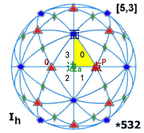
2. After using the coset enumeration algorithm to generate the vertex list, edge list, and face list, the articles do not explain how to determine the relationship between (n-1)-dimensional cells that compose the n-dimensional cells in the cell complex data structure. The generation method is not complicated. Let’s take finding the connections between vertices and edges as an example: First, generate the coset table of the entire reflection group (i.e., enumerate the cosets of the trivial subgroup {e}). Since each “fundamental region” corresponds one-to-one with the group elements of the reflection group, it also serves as a reflection table for all fundamental regions, where each region $i$ is reflected by $k$ to reach a new region $j$. Next, generate coset lists for vertices and edges. These lists record how each mirror reflects vertices/edges onto other vertices/edges. Vertices and edges are shared by multiple fundamental regions, and these shared vertices and edges are connected. Therefore, if we can obtain the index of vertices/edges/faces for each fundamental region, we can solve the connectivity problem between these points, lines, and faces. For example, in the diagram below, we see that edge a is shared by regions 0~3, and the vertices (P and Q) in these four regions form its endpoints.

Now, there’s still one problem left: How do we know the indices of vertices/edges in each fundamental region? First, all 0-indexed elements are the identity elements, meaning they belong to the initial fundamental region that does not undergo any reflection. All other fundamental regions are generated through a series of reflections. We just need to apply the reflection steps for each fundamental region to the vertices to find the new index for vertices in the corresponding region. By continuously referring to the coset table, we can complete this task.

Finally, let’s talk about the details of generating all the reflection steps for each fundamental region. We gradually build a table where the key is the region number, and the value is the sequence of reflection steps. First, the 0th region requires no reflection, so we write an empty sequence. Then, we scan the coset table row by row to generate new regions through reflection. If the new region already has a reflection sequence, we skip it. If not, we append the reflection we just performed to the current region’s sequence to generate the new reflection sequence.

Truncated Regular Polytope

Regular polyhedra are relatively simple, but how do we generate truncated, bitruncated, and edge-truncated polytopes? In the Wythoff construction for these polytopes, the initial vertex positions are no longer at the corners of the fundamental region. Some vertices are on the edges, and others lie inside the fundamental region. Additionally, the edges, faces, and cells of the polytope may have different shapes, and their symmetries differ. Therefore, it’s necessary to generate coset tables for the corresponding symmetry subgroups. Finally, we find the connection relationships through the fundamental regions, but since there are multiple types of elements of the same dimension, each coset enumeration assigns indices starting from 0. After adding them to the cell complex list, when indexing them for higher-dimensional cells, care must be taken to add an offset to the indices of the later-added elements. Below are some examples:

Truncated Regular Polyhedra

For example, for the truncated regular polytope formed by truncating the vertices of a 3D regular polyhedron (or for a 2D regular polygon tiling), we need to generate the coset lists of the symmetric subgroup generators for the following elements:

Label	Element	Symmetry Subgroup Generator
Ft	New Face Table (Original Vertex Position)	$f,e$
E	Original Edge Table	$f,v$
F	Original Face Table	$e,v$
V	New Vertex Table	$f$
Et	New Edge Table	$e$

We find that the truncated polytope has more elements than the regular polytope, and their centers are on the edges of the fundamental triangle instead of at the vertices. These elements have fewer symmetries, and the coset enumeration will generate more entries. After generating the cosets, we can find the connections between the regular polytope elements using the following algorithm (where A->B means recording a table of which elements in A form element B):

1. V->E, V->Et
2. Et->Ft, E->F, Et->F

After obtaining these connection relationships, we can construct the edge and face tables for the corresponding cell complex: The edge table is formed by merging the V->E and V->Et tables, and the face table is more complex. Since it stores index values, all new edges in the edge table are placed after the original edges. Specifically, the new edge 0 in the coset table corresponds to the original edge, so its index in the edge table will be the same as the original edge count. The face table will merge the E->F and Et->F tables.

Omnitruncated Polyhedra

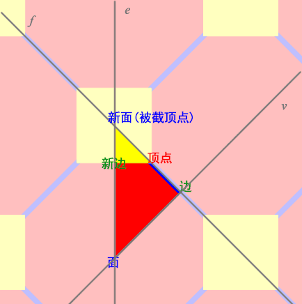
The omnitruncated polyhedra has its vertices completely inside the fundamental triangle and the least symmetry. The generated geometry is the most complex. We also draw the positions of each element within the fundamental triangle and list their connection relationship:

Label	Element	Symmetry Subgroup Generator
F	Original Face	$v,e$
Fe	Edge Cross Section	$f,v$
Fv	Vertex Cross Section	$e,v$
E1	Edge 1	$e$
E2	Edge 2	$v$
E3	Edge 3	$f$
V	Vertex	None

4D Truncated Regular Polytope
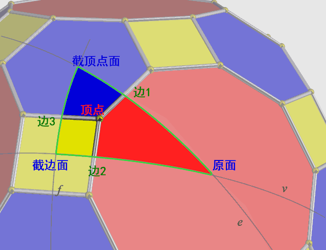
Since directly imagining and drawing the reflection hyperplanes on a 4D polytope is very difficult, we can instead draw the basic tetrahedra of the 3D regular polyhedron tiling to find these connection relationships, as they are the same as those in the 4D regular polytope. From the diagram, we can obtain the connection relationship table for the elements of the 4D truncated regular polytope:

The required connection relationships are as follows (where (A+B)->C means merging the tables A->C and B->C):

1. Edge Table: Vertex -> Edge, Vertex -> New Edge;
2. Face Table: New Edge -> New Face, (New Edge + Edge) -> Face;
3. Cell Table: New Face -> New Cell, (New Face + Face) -> Cell.

4D Bitruncated Regular Polytope

Similarly, we can derive the connection relationship table for the elements of the 4D bitruncated regular polytope. The new face 2 might not be obvious in the diagram; it represents the progressively larger octahedron created by bitruncation. After halving the edge-center face and continuing the bitruncation, two octahedra press against each other, transforming into a bitruncated octahedron. New face 2 is the “membrane” separating the two truncated cells, i.e., the quadrilateral face in the bitruncated octahedron.

The required connection relationships are as follows (where (A+B)->C means merging the tables A->C and B->C):

1. Edge Table: Vertex -> Edge 1, Vertex -> Edge 2;
2. Face Table: Edge 1 -> Face, Edge 2 -> New Face 2, (Edge 1 + Edge 2) -> New Face;
3. Cell Table: (New Face 1 + Face) -> Cell, (New Face 1 + New Face 2) -> New Cell.

Orientation of Cell Complexes

In rendering, triangles are often divided into front and back faces based on the order of vertices facing the camera to implement back-face culling or assign different materials to the front and back. This can be easily extended to distinguish the two orientations of a 4D tetrahedral cell by using the odd/even ordering of tetrahedral vertices. How can we assign orientation to a general cell complex? The concept from Homology on chain groups provides an idea: every n-dimensional face can have two possible orientations, similar to how vertices can have “positive” and “negative” states, line segments can have opposite directions, and polygons can be oriented based on the direction of their boundary edges (temporarily considered as clockwise/counterclockwise). The orientation of a body (cell) is determined by the orientation of its faces.

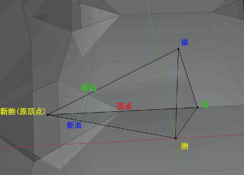
How is this recorded in computer program? For example, we might define all vertex orientations as positive, and for each line segment, we record the two endpoints where the first is positive and the second is negative. For polygons, we can define the orientation by ordering of edges, but for the 2D faces of a 3D cell, there is no meaningful ordering. It’s impossible to use an ordering to determine orientation. The general way to define orientation is to follow the construction method of the cell complex from low to high dimensions: the orientation of a higher-dimensional face depends on the orientation of its boundary. If it aligns with the default boundary orientation, it is marked as true; if not, it is marked as false. This gives us a Boolean orientation table, such as the one below for an oriented triangular prism, where the surface “vortex” direction appears counterclockwise from the outside.

Vertex：{(1,1,-1)₀,(-1,-1,-1)₁,(1,-1,-1)₂,(1,1,1)₃,(-1,-1,1)₄,(1,-1,1)₅}
Vertex Orientation: {True₀,True₁,True₂,True₃,True₄,True₅}
Edge：{(0,1)₀,(1,2)₁,(2,0)₂,(4,3)₃,(5,4)₄,(3,5)₅,(1,4)₆,(0,3)₇,(2,5)₈}
Edge Orientation: {(True,False)₀,(True,False)₁,(True,False)₂,(True,False)₃,(True,False)₄,(True,False)₅,(True,False)₆,(True,False)₇,(True,False)₈}
Face：{(0,1,2)₀,(3,4,5)₁,(0,3,6,7)₂,(1,4,6,8)₃,(2,5,7,8)₄}
Face Orientation: {(True,True,True)₀,(True,True,True)₁,(False,False,False,True)₂,(False,False,True,False)₃,(False,False,False,True)₄}
Cell：{(0,1,2,3,4)₀}
Cell Orientation: {(True,True,True,True,True)₀}

If you don’t understand, here’s an explanation using the orientation of face 2 (0, 3, 6, 7)₂: Following the swirl direction of the blue face 2 in the above image, its edges are 0, 7, 3, and 6. Among these edges, the direction that matches the swirl direction is the fourth one (7), which corresponds to True. The directions that don’t match are the first three (0, 3, 6), which correspond to False. Thus, the orientation is (False, False, False, True)₂.

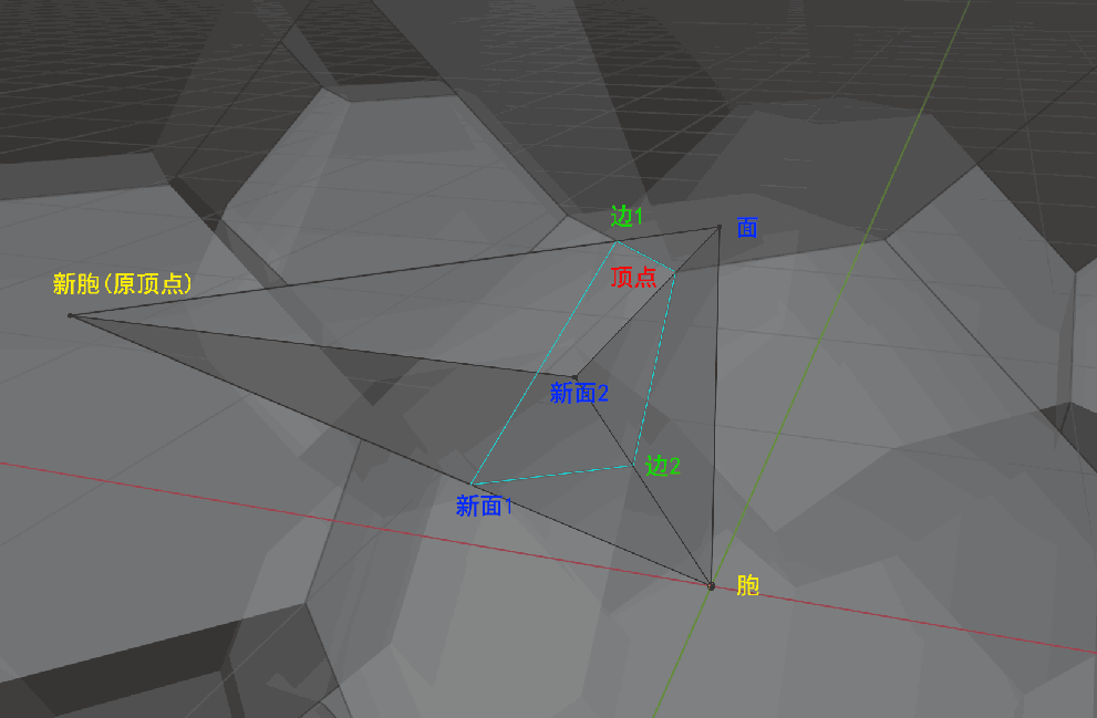
Note that the triangular prism only determines the orientation for three dimensions. The orientation of lower dimensions is irrelevant. The following diagram shows the same oriented triangular prism, but with some changes to the default orientations of certain 1D (edge 6) and 2D (face 4) elements in the data structure. (Modified oriented elements are highlighted in yellow, and changes in higher-dimensional orientation due to changes in lower-dimensional orientation are highlighted in cyan.)

Vertex：{(1,1,-1)₀,(-1,-1,-1)₁,(1,-1,-1)₂,(1,1,1)₃,(-1,-1,1)₄,(1,-1,1)₅}
Vertex Orientation: {True₀,True₁,True₂,True₃,True₄,True₅}
Edge：{(0,1)₀,(1,2)₁,(2,0)₂,(4,3)₃,(5,4)₄,(3,5)₅,(1,4)₆,(0,3)₇,(2,5)₈}
Edge Orientation: {(True,False)₀,(True,False)₁,(True,False)₂,(True,False)₃,(True,False)₄,(True,False)₅,(False,True)₆,(True,False)₇,(True,False)₈}
Face：{(0,1,2)₀,(3,4,5)₁,(0,3,6,7)₂,(1,4,6,8)₃,(2,5,7,8)₄}
Face Orientation: {(True,True,True)₀,(True,True,True)₁,(False,False,True,True)₂,(False,False,False,False)₃,(True,True,True,False)₄}
Cell：{(0,1,2,3,4)₀}
Cell Orientation: {(True,True,True,True,False)₀}

When designing the data structure, optimizations can be made. For instance, we could directly determine the orientation of edges and faces in order, without needing to record separate orientation tables for vertices, edges, and faces.

Now that we have a method for representing orientation, how do we generate this additional orientation information? Below, we introduce the algorithm for generating orientation data.

Unified Orientation Algorithm

Many times, we only have the basic data of a model without orientation information. For instance, the regular polytope data structure generated by the coset enumeration algorithm for symmetric groups doesn’t contain orientation information. In a polytope, once we specify the orientation of any face, the orientation of all other faces is automatically determined. The method for determining orientation is simple: the orientation of an edge in adjacent faces must be opposite. Using this principle, we can gradually expand outward from the known oriented faces, determining the orientations of other faces by connecting adjacent ones. The same principle applies to polytopes: the orientation of the shared face between two adjacent cells is opposite in each cell.

In fact, as long as the cell complex has a local manifold structure (i.e., n-1 dimensional cells are shared by only two n-dimensional cells), orientation can be determined using the propagation algorithm described earlier. There is one exception, though: in a Möbius strip or other non-orientable manifolds, the propagation algorithm will find that the orientations don’t match after one full cycle, making it impossible to perform back-face culling for rendering these one-sided surfaces.

The unified orientation algorithm essentially applies orientation after constructing the model. But how can we use existing orientation information when modeling on a known oriented shape to determine the orientation of newly constructed shapes? Below, we will look at how to handle orientation information in coneification and direct product operations.

Orientation of Pyramids

A pyramid consists of a base and side faces formed by connecting the apex to the faces of the base. We denote the pyramid constructed from an $n$-dimensional cell $A$ as $\widehat{A}$. Note that once the orientation of $A$ is given, the orientation of the $(n+1)$-dimensional pyramid $\widehat{A}$ does not follow directly from it. We must assign an orientation to $\widehat{A}$ explicitly. A natural choice is to let the base retain the same orientation as $A$. This provides a consistent convention for recursively building oriented pyramids from lower to higher dimensions.

The side faces (i.e., the pyramids over the boundary faces of $A$) will inherit their orientation from $A$ as well, but with a possible sign factor. We introduce an undetermined coefficient $a(n)$ (taking values ±1) to account for this, and write the boundary of the pyramid as:

$$
\partial(\widehat{A}) = A + a(n), \widehat{\partial A}
$$

Here, $A$ is the base, and $\widehat{\partial A}$ represents the side faces formed by pyramidal construction on each face of $A$.

Since the boundary must itself be a closed shape, applying the boundary operator again gives:

$$
0 = \partial^2(\widehat{A}) = \partial A + a(n)\left( \partial A + a(n-1)\widehat{\partial \partial A} \right)$$Noting that $\widehat{\partial\partial A} = 0$, this simplifies to:$$0 = \partial A(1 + a(n)) \Rightarrow a(n) = -1$$Therefore, we obtain the final formula:$$\partial(\widehat{A}) = A - \widehat{\partial A}$$

Orientation of Direct Products

We know the formula for the boundary of a direct product shape is:
$$\partial (A \times B) = \partial A \times B + A \times \partial B$$
However, this formula doesn’t account for orientation, so we need to modify it. We introduce unknowns $a$ and $b$, both of which can only take values ±1, and depend on the dimensions of the shapes. Let $\dim{A} = m$ and $\dim{B} = n$, so $a$ and $b$ are functions of $m$ and $n$, and can be written as:
$$\partial (A \times B) = a(m,n)\partial A \times B + b(m,n)A \times \partial B$$
Since there are always two possible orientations, we can arbitrarily select one direction to define the orientation of the direct product shape of the two oriented shapes. Here, we choose $b(m,n) = 1$, meaning that after the direct product, the orientation of $A$ remains the same as its original orientation. Thus, we have:
$$\partial (A \times B) = a(m,n)\partial A \times B + A \times \partial B$$
The boundary must be closed, so:
$$\partial^2 (A \times B) = 0 = a(m,n)\partial(\partial A \times B) + \partial(A \times \partial B)$$
Using $\partial^2A = 0$ and $\partial^2B = 0$, and knowing that $\dim(\partial A) = m-1$ and $\dim(\partial B) = n-1$, we simplify to:
$$0 = a(m,n)(\partial A \times \partial B) + a(m,n-1)(\partial A \times \partial B)$$
Since $A$ and $B$ can be any shape, for this equation to hold true for all cases, we must have $a(m,n) = -a(m,n-1)$. To allow the recursive formula to work smoothly, we need to provide an initial value. When $B$ is a 0-dimensional point, we want it to behave like a scalar and not alter the orientation of shape $A$, so we define $a(m,0) = 1$. Thus, we obtain:$$a(m,n) = (-1)^n$$

Simplex Decomposition of Cell Complexes

In the rendering section, we have already mentioned an algorithm for decomposing polygons into triangles: simply choose any vertex and connect it to the other non-adjacent vertices. How can we apply this to tetrahedral decomposition of a polyhedron or higher-dimensional polytopes into 5-cells (a form of simplex decomposition)? We can use the following algorithm:

Decomposing an $n$-dimensional complex is recursive: first, to decompose an $n$-dimensional complex, we need to decompose its $(n-1)$-dimensional faces. For any $n$-dimensional cell to be decomposed, we assume all its $(n-1)$-dimensional faces have already been decomposed into $(n-1)$-dimensional simplices. Then, we choose a point and, using the cell complex data structure, we can easily find all $(n-1)$-dimensional faces containing the point. We ignore the simplices that were already decomposed from them, and then we perform a coneification operation to create $n$-dimensional simplices by connecting the point to the simplices formed by the remaining $(n-1)$-dimensional faces, completing the decomposition. This algorithm is a generalization of drawing diagonals in polygons, but we avoid simplices that share the vertex to avoid generating degenerate simplices with zero volume. This algorithm also retains the orientation information of the cell complex to be decomposed, as it only involves coneification, for which we already described how to handle the orientation to make sure the cone’s orientation is consistent with the base.

It is worth noting that recording the information for simplices created by the decomposition does not require edge tables, face tables, etc. All vertices of a simplex are connected pairwise, and any three points form a triangular face, so we only need to record the vertex indices. The odd/even ordering of the vertices completely determines the orientation of the simplex, and no additional orientation table is required. During rendering, back-face culling can be easily determined by forming a determinant with the coordinates of the four vertices of the tetrahedron and checking the sign of the determinant to determine whether the tetrahedron is facing the camera or not.

4D Basic Cell Format

We know that the basic elements of a typical 3D mesh model are triangle faces, but many modelers prefer using quadrilaterals because they better fit the logic of modeling and topology. In a similar way, in four-dimensional modeling, the basic cells are tetrahedra, but a cube or other six-faced polyhedron must be decomposed into five tetrahedra. Therefore, directly supporting hexahedral meshes is quite necessary for four-dimensional modeling. Unlike two-dimensional space, where polygons between triangles and quadrilaterals don’t exist, in three dimensions, apart from tetrahedra and hexahedra, could there be other basic cells? Many engineering applications in our world use finite element methods for simulation calculations, which require polytope decompositions. For example, the multi-physics finite element analysis software COMSOL supports tetrahedra, triangular prisms, pyramidal quadrilaterals, and hexahedra as its four basic units: (Here is the official COMSOL Blog introducing different decompositions)

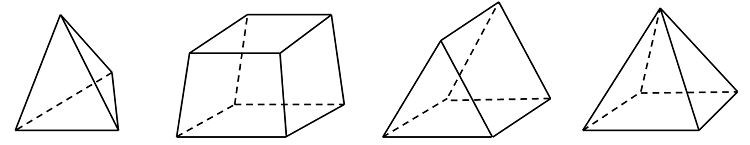
These four elements, when decomposed in four-dimensional modeling, can be obtained by pyramid construction or extruding a 3D mesh made of triangles or quadrilaterals. Although Tesserxel currently only supports tetrahedra rendering, we can follow the same format used for the 3D Wavefront obj file (.obj) to specify the vertex order for these four elements, representing and recording cells (and orientations). Using these cells, we can construct complex four-dimensional mesh models.

Below is a traditional 3D OBJ file that records one triangular face and one quadrilateral face:

# Lines starting with '#' are comments

# 'v' denotes vertex data; the following five lines define the coordinates of five vertices
v -1 -1 0
v 1 -1 0
v 1 1 0
v 2 1 0
v 2 -1 0

# 'f' denotes face data; the following lines define one triangular face and one quadrilateral face
# The order of the vertices determines orientation
f 1 3 2
f 2 3 4 5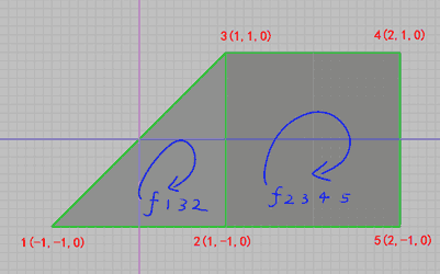

Similarly, we introduce: t for tetrahedrons, tp for triangular prisms, qp for quadrangular pyramids, h for hexahedrons. The following cell elements are denoted as:

t 1 2 3 4
tp 5 6 7 8 9 10
qp 11 12 13 14 15
h 16 17 18 19 20 21 22 23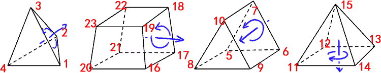

We can also define their orientation as follows:

1. In the 3D space containing the tetrahedron, use the right-hand rule on the first three vertices. If the resulting normal points toward the fourth vertex, the tetrahedron’s normal points out of the 3D screen; if it points away, the normal points into the screen.
2. For triangular prisms, if the right-hand rule applied to the bottom triangle gives a normal that points toward the opposite triangle, then the prism’s normal points outward; otherwise, inward.
3. For quadrangular pyramids, the first four vertices form the base. If the right-hand rule on this base gives a normal pointing toward the apex (fifth vertex), the pyramid points outward; otherwise, inward.
4. For hexahedrons, the first four vertices define the bottom face. If the right-hand rule gives a normal toward the top face, then the normal points outward; otherwise, inward.

Explanation: The term “right-hand” refers to a real 3D human hand. To apply this in 4D, we imagine placing the right hand into a 3D subspace of the 4D space. From one side of this 3D subspace, a 4D observer sees the right hand as normal; from the opposite side, it’s seen as a mirrored left hand — just like how text appears reversed when viewed through a sheet of paper. Thus, handedness is relative in 4D. The orientation described above is well-defined: no matter which side the 4D observer is on, the direction of the normal vector remains consistent. From the diagram, note that the triangular prism is oriented outward, while the other three shapes point inward.

Now, it seems like we can use these notations to represent arbitrarily complex 4D scenes. However, it’s not that simple. All of the above assumes that the $n$-dimensional shape being decomposed is flat in its $n$-dimensional space: each face must lie in a $(n-1)$-dimensional hyperplane, and the full shape must lie in an $n$-dimensional hyperplane. For curved surfaces, this condition can easily be violated, and the above decomposition methods may fail. We’ll explore that in the next section.

Validity of Decompositions

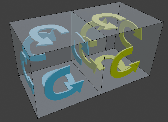
Our current decomposition algorithm has issues with non-coplanar geometry. For example, if we decompose two adjacent hexahedrons into tetrahedrons, but the shared quadrilateral face is not planar and both sides use different triangulations, the result can be overlapping tetrahedra or hollow gaps.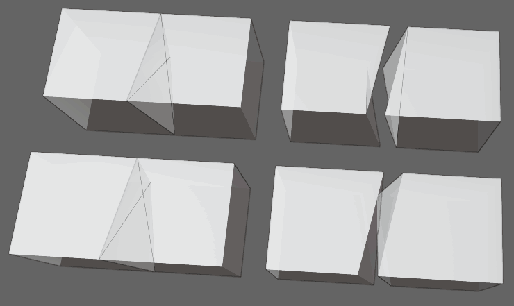

Such overlaps and gaps affect rendering. This issue, for instance, exists in the rotating monkey-head (Suzane) scene in Tesserxel. A well-formed decomposition must be consistent on shared boundaries. For example, a good decomposition of a hexahedral mesh uses staggered diagonals on adjacent faces (right), not the same diagonal direction (left).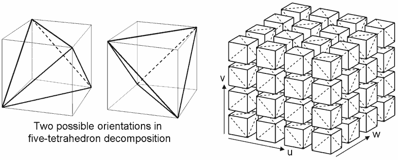

So, how do we find a best-fit decomposition that meets these criteria for any 4D cell complex? Unfortunately, there’s no known polynomial-time algorithm. Worse, some concave polyhedra can’t even be tetrahedralized without adding new vertices. One such shape is the Schönhardt polyhedron, a twisted triangular prism where all side faces are triangulated the same way.

This also shows that a given triangulation of a triangular prism’s sides may not yield a valid decomposition. Below are all $2^3 = 8$ combinations of side-face triangulations; only the green ones yield valid tetrahedralizations.

Hexahedrons are more complex. Each of the six faces has two triangulation choices, giving $2^6 = 64$ total. Of these, 46 (a–e) are valid; 18 (f–g) are invalid.

To check validity, there’s a useful trick: if three face diagonals converge at one vertex, the decomposition is valid. You can divide the hexahedron into three quadrangular pyramids, and any pyramid can be further tetrahedralized. However, this is only a sufficient condition, not a necessary one — case (b) is the only counterexample.

To prove a decomposition is invalid: if it exists, then all triangular faces must be faces of some tetrahedron. Try finding a fourth vertex that, along with a triangle, makes a valid tetrahedron. If no such vertex exists for any triangle, the decomposition is invalid.

Among all valid decompositions, only two in case (a) produce just five tetrahedra — the most efficient. All others produce six. So, if possible, we prefer those two to reduce rendering overhead.

Lastly, quadrangular pyramids are the simplest: they have only two triangulations, both valid, both yielding two tetrahedra.

A 4D mesh may consist of a mix of these cell types. To avoid overlaps and cracks caused by non-coplanar quads, we must:

1. Specify a triangulation for each quadrilateral face (choose a diagonal).
2. Ensure each cell uses a valid decomposition.

We can use a greedy strategy: since hexahedrons are most likely to be invalid (as shown in the statistics), we first select an optimal decomposition for all hexahedrons. Then, we propagate consistent triangulations to adjacent cells. If neighboring cells are of mixed types, we prioritize in this order: hexahedron > triangular prism > quadrangular pyramid. For each cell, aside from the two optimal hexahedral decompositions, the rest are randomly chosen. If no valid decomposition is found, we backtrack and try a different choice.

Youtuber Codeparade encountered the same problem when designing tree models for the game 4D Golf. He noticed that different triangulations of spatial quads can cause gaps. He proved that finding a valid triangulation for prism meshes is NP-complete. Specifically, if the 3D base is a mesh of triangles, these extrude into triangular prisms. Each rectangular side face can be triangulated in two ways. However, as shown earlier, not all choices lead to valid tetrahedralizations. Codeparade converted the diagonal-choosing problem into a graph-coloring problem, thus proving it’s NP-complete.
For details, see his video.

These examples show how hard the tetrahedralization problem really is. Even finding any valid decomposition (not necessarily optimal) is difficult. This article only discussed hexahedrons, triangular prisms, and quadrangular pyramids. For more complex 3D cells — like the dodecahedra in the 120-cell — things get even harder. How do we decompose a distorted 120-cell to avoid cracks due to non-coplanar faces? How do we tetrahedralize arbitrary implicit surface cells with diverse shapes?

Fortunately, we have a brute-force fallback:

• For any 2D face: triangulate it arbitrarily.
• For any 3D cell: add a central point (cell center) and connect it to all triangles of the faces.

This guarantees a valid tetrahedralization — though it requires extra vertices and produces more tetrahedra.