Explaining the "Dimensions" Trailer
The last episode of the “Dimensions” series is a trailer: Dimensions II — its content is not the later released “Chaos”, but the latest research results of one of the “Dimensions” creators — mathematician Étienne Ghys. This content is even more profound, and I estimate they probably won’t release this episode. I found an article on the website of Jos Leys, another creator of “Dimensions”, introducing the graphics that appear in the trailer (i.e., Étienne Ghys’s latest research results):
Please first read the original article by Jos Leys
Here is my Lattice Space 4D Online Viewer
(I’ve always wondered why the trajectories of the modular dynamical system I drew are so close to the discriminant trefoil knot, I’ve checked the code many times but couldn’t find the reason)
If you’re interested and want to go deeper, you can read some books about elliptic functions and modular forms. I recommend Pan Chengdong’s “Introduction to Modular Forms” (there’s a PDF online, I can understand the first three chapters, but not the later ones)
Below are my understanding and supplements for some difficult parts I encountered while reading this article.
Lorenz Attractor
If you cannot understand or want to know more about the Lorenz attractor, please watch another video series by the “Dimensions” creators: “Chaos“. If we really want to do quantitative analysis, it would definitely involve extensive formula derivations, so we won’t discuss it here.
Seifert Surface
Seifert surfaces are very interesting: they refer to surfaces bounded by knots or links. For example, the Seifert surface on the Hopf link: 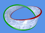
Surfaces are divided into one-sided surfaces (non-orientable) and two-sided surfaces (orientable). The most famous example of a one-sided surface is the Möbius strip. The boundary of a Möbius strip is a circle, and of course, a circle can be viewed as a trivial knot. So, there are at least two types of Seifert surfaces with a circle as boundary: 
Where I’ve colored the outside of the knot means this surface is like looking at a balloon with a hole from the inside, flip it over and twist it half a turn to get a regular disk.
Let’s look at the trefoil knot: we have these types of Seifert surfaces: Note that the two on the right are also trefoil knots, just with different projections. The shape of the $\Delta = 0$ curve when constructing the “template” later looks like this. 
We can use the coloring method to determine whether these Seifert surfaces are one-sided: the surface at each “crossing” of the knot appears to be twisted 180°, so after passing through a crossing, the front and back should be swapped. If we can alternately color the entire surface with two colors (one for each side), it means it’s a two-sided surface, otherwise it’s one-sided.
Using this method, we find that only the first surface is two-sided — it’s the surface in four-dimensional space mentioned in Josleys’ article!
Matrices
The lattice animation in the modular dynamical system is the most spectacular. To understand the specific description of this construction in the article, you first need to have concepts of linear algebra matrices, eigenvalues, and similar matrices. These concepts are not complex and can be found online or in any linear algebra textbook. The only thing I want to mention is the method of decomposing modular matrices into U and V matrices: left-multiplying a matrix by a U or V matrix corresponds to simple column operations on this matrix: adding one column to another. So we work backwards: each operation subtracts the smaller column from the larger column, and we can always reach the identity matrix. If it’s right multiplication, it corresponds to row operations, and we can eventually find the formula for decomposition into U and V matrices.
Lattice Space Structure Diagram
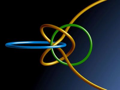
$g_2$ and $g_3$ are core parameters describing lattices, and they are also important quantities in modular form theory. But their definitions are all infinite sums over lattice points, and understanding them seems to involve complex advanced mathematical operations. We don’t plan to delve too deeply into this content. Below, we’ll maximize our understanding from the ready-made clues given in the article about which lattices the points in lattice space actually correspond to:
First, the article mentions the two circles $g_2 = 0$ and $g_3 = 0$, which are square lattices and regular hexagonal lattices respectively. Then we have a yellow trefoil knot corresponding to the curve $\Delta = 0$. The article also tells us that when $\Delta = 0$, $(g_2, g_3)$ doesn’t correspond to any lattice, which means something must happen near the curve $\Delta = 0$. Calculations show that if a lattice is very “flat”, its $|\Delta|$ will be very small. If it’s infinitely flat, its $\Delta = 0$, but of course infinitely flat doesn’t exist.
Why does $\Delta = 0$ correspond to a trefoil knot?
Generally, when we rotate a lattice half a turn, the lattice coincides with the original. During this process, the parameter $g_2$ rotates in the complex plane at four times the angular velocity (because the definition of g_2 contains the fourth power of lattice points, multiplying the argument by 4), and $g_3$ rotates in the complex plane at six times the angular velocity. These two rotations combine to form the total motion in lattice space: double rotation at unequal angles. CFY’s this article has already analyzed this kind of motion, and its trajectory is a trefoil knot.
This motion fills the four-dimensional sphere with trefoil knots. These trefoil knots together with two circles ($g_2 = 0$, $g_3 = 0$) fill the entire four-dimensional hypersphere, and we get another fiber bundle!
From here we see that infinitely flat lattices are also treated as ordinary lattice rotations, it’s just a very ordinary trefoil knot in the fiber bundle.
Now let’s mark the structures we already know in two views: 
Later in the article, when constructing the “template”, it gives us information: a certain diameter of the circle where all regular hexagonal lattices are located ($g_3 = 0$) consists of rhombuses with horizontal diagonals, with vertex angles varying between 60° and 120°. What if the vertex angle exceeds this range of 60° to 120°? We conjecture that extending this diameter outward corresponds to those points. Extend infinitely? We’ll “hit” the line $\Delta = 0$: it corresponds to very flat rhombuses with vertex angles of 0° and 180°. 
If we pass through $\Delta = 0$ and continue extending, we’ll eventually extend to infinity: that point corresponds to a square lattice. From $\Delta = 0$ to infinity corresponds to infinitely flat rhombuses to square lattices. What’s going on in this process? Actually, the moment we pass through $\Delta = 0$, the lattice has already changed from a rhombus to a rectangle! Because when infinitely flat, you can’t distinguish between rectangles and rhombuses. The red extension line corresponds to the compression and stretching of rectangles. 
Let’s look at this extension line from another perspective: 
We find that points on the red part correspond to all rectangles with arbitrary aspect ratios and sides parallel to the real and imaginary axes. If we rotate them, we get the set of all rectangles. Remember that the trajectory after rotation is a trefoil knot? The union of infinitely many trefoil knots obtained by rotating these points gives us a new Seifert surface of the trefoil knot (purple in the figure below) — this is the set of all rectangular lattices — it’s also a one-sided surface like the Möbius strip, except the paper strip is twisted one and a half turns before gluing! (The Möbius strip is half a turn) 
Geodesics in Hyperbolic Space
Finally, let’s look at another representation method for lattice space: not only do we ignore the size of the lattice, but we also ignore the lattice direction (for example, considering all square lattices as the same). We have another visualization method: use the complex number $\tau = w_2/w_1$ to represent a lattice. But when we exchange the positions of $w_2$ and $w_1$ to get $1/\tau = w_1/w_2$, it’s also a value of $\tau$, but only one of these two values falls in the upper half-plane ($Im(\tau) > 0$). So we add a restriction here: we will only discuss in the upper half-plane from now on. But there are infinitely many ways to choose the complex numbers $w_2$ and $w_1$, so we’ll get infinitely many values of $\tau$. But we can generally always find a unique value of $\tau$ in the region $|Re(\tau)| \le \frac{1}{2}, |\tau| \ge 1$. We call this region the fundamental domain. How do points in other regions differ from points in this region? Their choice of $w_1$ and $w_2$ differs by a modular matrix — a second-order integer matrix with determinant 1. Reflected in the complex number $\tau = w_2/w_1$, they differ by some Möbius matrices (which have nothing to do with the Möbius strip). For specific details, see the PDF introducing it. For example, the infinitely flat lattice with $\Delta = 0$ is at $\tau = +i\infty$, the square lattice is at $\tau = i$, and the regular hexagonal lattice is at $\tau = r = 1/2 + i\sqrt{3}/2$. 
The modular dynamical system reflected in the upper half-plane of $\tau$ consists of arcs with centers on the real axis. We can think of this as a curved two-dimensional space: all the arcs you see with centers on the real axis are “straight lines”, it’s just an illusion created by the curved two-dimensional space — because our flat space cannot perfectly express the curved two-dimensional space, just like when we use stereographic projection to draw things on a sphere, the image is distorted; in this curved two-dimensional space, every curved-edge triangle is the same size. The triangles near the real axis look small, which is also an illusion created by the curvature — this is hyperbolic space! These “straight lines” we call “geodesics” (geodesics were discussed in the mathematical film “Chaos”). Hyperbolic space doesn’t satisfy “only one parallel line can be drawn through a point outside a line“, it can draw infinitely many parallel lines! What is parallel? In two dimensions, not intersecting is parallel. Can you find examples in the above figure that negate “only one parallel line can be drawn through a point outside a line”?
Hyperbolic space appeared as early as Episode 2 of “Dimensions”: 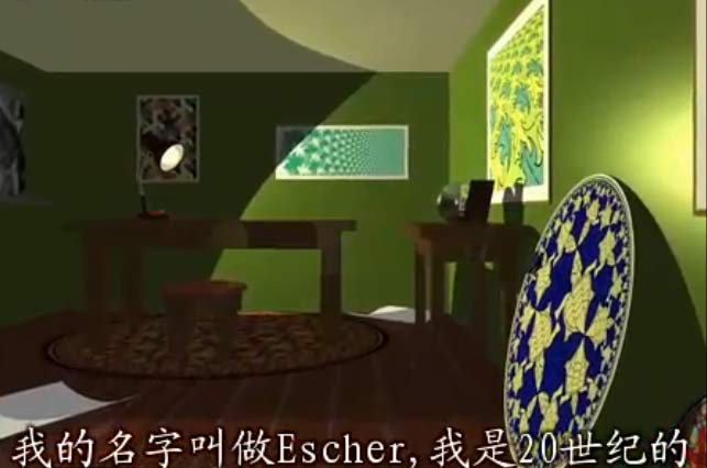
Notice that disk and the pattern on the wall? That’s a work by Escher inspired by the geometry of hyperbolic space. We will discuss hyperbolic space in detail later.