The Magical Hyperbolic World

In my old article from years ago “Hyperbolic Space - Mathematical Art“, I introduced the mathematical geometric concept of hyperbolic space, and recently “Minkowski Space and Constant Curvature Spaces“ also mentioned it again. Similar to the four-dimensional space series and four-dimensional world series, this article will discuss some interesting physical phenomena in the hyperbolic space world. On this blog I’ve spent considerable ink introducing an imaginary four-dimensional world, while also introducing worlds constructed through non-Euclidean geometry like the hyperbolic space world, p-norm worlds, and even pure thought experiments like Inverse Earth, Electron-Deficient Planet vs Electron-Rich Planet… Starting from this article, I’m opening a special “Strange Worlds” series to introduce some imaginative worlds beyond the four-dimensional world.

Since the first article mainly showed readers hyperbolic space visually, and the latter article focused on construction methods in Minkowski space, neither systematically introduced hyperbolic geometry. Therefore, we’ll first supplement some geometric properties not mentioned before, then based on this describe an imaginary hyperbolic universe, exploring the mechanics, astronomy within it…

Lines, Circles, Horocycles and Equidistant Curves

Hyperbolic space is infinitely large. Although defining hyperbolic space on a hyperboloid in 3D Minkowski space is the most direct approach, the Poincaré disk model is visually the most convenient. The property that objects appear smaller as they approach the edge of the Poincaré disk should already be familiar to readers (see “Hyperbolic Space - Mathematical Art“). I highly recommend everyone play “Hyperrogue“, a 2D hyperbolic space adventure game - I even think if you’re doing mathematical research on non-Euclidean geometry and haven’t played this game, that’s a real shame. Let’s look at some simple geometric concepts:

Lines

We know that one of the most distinctive features of hyperbolic space is that it doesn’t satisfy Euclid’s fifth postulate, which I won’t elaborate on here. As mentioned in previous articles, in 3D Minkowski space, the intersection of a plane through the origin with the hyperboloid forms a line, similar to how a plane through the center of a sphere intersects the sphere to get a great circle (geodesic). Lines (geodesics) in hyperbolic space have this property in the Poincaré disk projection: they are all circular arcs that intersect the disk boundary at right angles.

The following figure reflects the most important property of hyperbolic space regarding the parallel postulate: through a given point, there are infinitely many lines parallel to line $a$ (such as $d$, $e$, $f$). The infinite Euclidean plane is much larger than a closed sphere - don’t be fooled by its Poincaré projection being a finite circle. In a certain sense, the hyperbolic world is much larger than the Euclidean plane! For example, between parallel lines $a$ and $b$, we can accommodate new parallel line $c$ in ways unimaginable in Euclidean space!

Circles

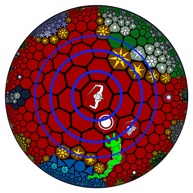
We can also define circles in hyperbolic space: still the set of points at a constant distance from a given point. Note that the radius here becomes a geodesic segment (i.e., the lines defined above), and the length of the geodesic segment (radius) is also calculated using hyperbolic distance. Note that the Poincaré projection shrinks figures near the boundary, which explains why the center of the circle in the figure appears in a lower position.

Due to the divergent nature of parallel lines in the hyperbolic world, the circumference and area of hyperbolic circles grow exponentially with radius! For example, the three circles below with radii of 1/2/3 tiles pass through 7/14/28 tiles respectively, as can be counted in the figure - this is a geometric sequence. If the circle’s radius exceeds ten tiles, the circumference will reach tens of thousands of tiles! From the Poincaré disk projection, we can see that the closer the circle is to the boundary, the more area tiles it can “contain”.

Similar to lines, here are circles in two models:

1. General circles on a sphere are obtained by intersecting the sphere with planes not passing through the center. Similarly, we can intersect the hyperboloid with planes not passing through the origin, but unlike the spherical case, the intersection may or may not be closed. If the intersection is a closed figure, then it’s a circle. Why? Obviously, if we cut the surface with planes perpendicular to the hyperboloid’s axis of symmetry, we get a series of circles. It can be verified that they are also circles under the Minkowski metric. For any plane, we can always rotate it to be perpendicular to the hyperboloid’s axis through hyperbolic rotation, thus verifying that these closed figures are all circles.
2. Circles in hyperbolic geometry remain circles after Poincaré disk projection, similar to the circle-preserving property of stereographic projection, but after projection the circle’s center often no longer coincides with its actual position.

Horocycles

The hyperbolic world is amazing because it has figures impossible in Euclidean space. For example, horocycles: circles with centers at infinity and infinite radius. In Euclidean space, a circle with infinite radius becomes a line, but in the hyperbolic world, horocycles have curvature. Here are some properties of horocycles:

1. Horocycles in the Poincaré disk projection are tangent to the disk boundary. Note that don’t think that walking in opposite directions from a horocycle will eventually bring you closer together - this is just an illusion from projection compression at the boundary. In fact, you’ll only get farther apart.
2. Horocycles, like circles, are highly symmetric figures, and all horocycles have the same curvature, so in this sense they are all the same size. (The figure below is clearly a Smith chart)

3. In 3D Minkowski space, horocycles are parabolas obtained by intersecting planes parallel to any asymptotic line of the hyperboloid.

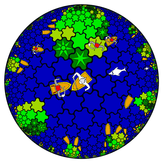
Without directional guidance, it’s very difficult to go deep into a horocycle’s interior. You must head directly toward the infinitely distant center - with even slight deviation, you’ll soon walk out of the horocycle! The islands in this biome in “Hyperrogue” are horocycles. I suggest everyone experience it firsthand. There are scattered compasses pointing to the horocycle’s center, and only by following their guidance can you continue deeper into the island.

Equidistant Curves/Hypercycles

We know that the larger a circle’s radius, the smaller its curvature. The same is true in hyperbolic space, but the existence of horocycle curvature indicates there are figures with even less curvature than horocycles but that aren’t lines. Actually, it’s not hard to imagine - following the progression from circles to horocycles, such curves should appear in the Poincaré projection as circular arcs intersecting the boundary. Their centers are even more distant than infinity - a transcendent existence beyond infinity! These are equidistant curves, also called hypercycles. We can actually define them without invoking infinity. We know that the distance between two initially parallel lines grows larger and larger. If we forcibly create a “parallel” line that maintains constant distance from a given line, we get an equidistant curve! We call this line the axis of the equidistant curve, and the distance from the equidistant curve to the line is called the radius of the equidistant curve. When the radius is 0, the equidistant curve coincides with the line. The larger the radius, the greater the curvature. An equidistant curve with infinite radius becomes a horocycle!

On a sphere, the equidistant curves of a line are circles, which are shorter than the line. Similarly, equidistant curves in hyperbolic space are longer than their parallel lines. In the Hyperrogue game, there’s a biome where tiles fall after the player walks on them. When enemies chase players fleeing along geodesics, they can only walk on equidistant curves. Since equidistant curves are longer than lines, it doesn’t take long before enemies can’t catch up with players.

In 3D Minkowski space, intersecting the hyperboloid with planes can yield closed ellipses, parabolas, and hyperbolas, which correspond to circles, horocycles, and equidistant curves respectively. Note there’s an exception: if the plane intersecting the hyperboloid passes through the origin (in which case it also yields a hyperbola), the result is not an equidistant curve but a geodesic.

Conception of a Hyperbolic Universe

Although we’ve been discussing 2D hyperbolic worlds, these geometric motion laws still hold in higher-dimensional hyperbolic spaces. The worldview of the Hyperrogue game is actually players moving on an infinite hyperbolic plane. Although the game doesn’t involve a third dimension, from the top-down view of the characters, the Hyperrogue world does have a third dimension - you just can’t control character movement in the height direction. The analogy in Euclidean space would be players walking on infinite flat ground. However, the real world has no infinite ground - we live on Earth. So, can we construct hyperbolic planets and hyperbolic universes?

Yes! Let’s try to describe a 3D hyperbolic universe: similar to our world, it has countless galaxies, there might be a spherical planet with suitable conditions that could nurture life… This story wouldn’t differ from our real world. Actually, the most obvious characteristic of a hyperbolic universe is curvature. If the curvature is small enough and the range of activity is also small, we can hardly distinguish between flat space and hyperbolic space. Therefore, we can only assume this universe has very large curvature, as large as the scale in the Hyperrogue world, which would bring some interesting effects:

1. Navigation in the hyperbolic world is difficult, it’s easy to lose direction. (You should have already experienced this in the Hyperrogue game)
2. A planet with a small radius has an abnormally large surface area and volume, almost astronomical numbers.

Inspired by the game, let’s imagine some bolder things: could there exist infinitely large planets shaped like horocycles? Or even more crazy, could even infinite half-space planets exist? In a flat universe, if a planet occupies half of the entire universe, this universe can at most accommodate one more such planet. Not so in the hyperbolic world - it can simultaneously contain infinitely many half-space planets! A fatal problem is the gravity of these planets - if calculated to be infinite, it becomes meaningless. Next, we’ll derive step by step the (classical) law of universal gravitation in a hyperbolic universe! Before exploring this complex problem, let’s first look at some simple laws of Newtonian mechanics in the hyperbolic world.

Rigid Body Motion in the Hyperbolic World

There are so many transformations in the world, such as translation, rotation, scaling, stretching, twisting, flipping, etc. But rigid objects in daily life can only perform translation and rotation - why is this? The answer is that only translation and rotation transformations in space can maintain constant distances between points within a rigid body during continuous motion.

Translation

In Euclidean geometry, when a rigid body translates, the motion trajectories of all points are parallel lines, thus maintaining constant distances. What about in hyperbolic space? Parallel lines diverge and can’t maintain distance - no ideas? We can first look at spherical geometry: imagine a 2D object moving with “uniform linear” motion in a 2D spherical world. Its center of mass trajectory is a great circle on the sphere. Let’s consider this great circle as the equator - then points north of the equator have trajectories that are small circles, no longer geodesics! Small circles have curvature, meaning they must have experienced forces to “deviate” from geodesics - if they followed geodesics, various parts of the object would squeeze together vertically. The elastic force resisting compression acts as the centripetal force for following small circles, keeping the object from deforming.

Hyperbolic space has the opposite effect of spherical space. For the ends of a moving object in hyperbolic space to maintain constant distance from the center of mass, they must follow equidistant curves. Equidistant curves have curvature, so they experience forces stretching perpendicular to the direction of motion. This can also be explained by the previously mentioned divergence of geodesics. These facts indicate that object motion in hyperbolic/spherical worlds has absolute velocity, which can be calculated by measuring internal stress within the object. Additionally, objects in hyperbolic space have a speed limit determined by structural strength - beyond this speed, objects will disintegrate. This is a tidal force effect caused by curvature, similar to the Roche limit in celestial mechanics (in general relativity, isn’t gravity also a curvature effect?).

Feel a bit disappointed that this world has an absolute rest reference frame? Actually, considering relativity does solve this problem. The relativistic version of hyperbolic space is the anti-de Sitter spacetime mentioned in previous articles, which I won’t discuss here.

Rotation

Everyone knows rotation requires sufficiently strong centripetal force, otherwise parts of the object will be flung away. Therefore, rotational angular velocity is an absolute physical quantity, and there’s also a rotation speed limit related to material structure. The same applies to hyperbolic and spherical worlds. Regarding rotation, hyperbolic space has something special: ideal rotation - a rotation with center at infinity, where all participating points have trajectories that are horocycles! Horocycles have finite curvature, so the centripetal force needed for this rotation can actually be provided. Just note that at the same angular velocity, the relationship between linear velocity and radius is also exponential.

Mathematically, it can be proven that rigid transformations in hyperbolic space fall into only three categories: hyperbolic, elliptic, and parabolic, corresponding to translation, rotation, and ideal rotation respectively. This website has detailed analysis of rigid transformations in hyperbolic space, with beautiful illustrations:

Finally, let me remind everyone: rigid motion in spherical geometry has only one type - rotation, because translation along the equator is exactly the same as rotation around the north and south poles.

Fields and Gauss’s Theorem

Now let’s explore possible shapes and gravity of hyperbolic planets: Under Newtonian mechanics, gravitational fields are highly similar to electromagnetic fields. For example, in 3D flat space they both decay as inverse square, in 4D flat space they both decay as inverse cube… The source is conservation of total “field line quantity” and the “dilution effect” of space on field lines, which was mentioned in the derivation of gravity in the four-dimensional world. Let’s first derive the electric field strength $E$ as a function of distance $r$, $E(r)$, for a point charge $q$ in a 2D flat world. Draw two concentric circles with radii $r_1$ and $r_2$. By symmetry, all electric field lines emitted by charge $q$ pass through both concentric circles. This flux can be obtained by multiplying field strength by circumference, so we have $2\pi r_1 E(r_1)=2\pi r_2 E(r_2)$, i.e., $2\pi r E(r)$ is constant, yielding that $E(r)$ is inversely proportional to distance.

Now let’s solve the point charge electric field problem in hyperbolic space by following the same pattern. As long as we know the circumference formula for circles, the electric field is diluted by these circumferences that grow longer with distance. As mentioned before, circumference in hyperbolic space grows exponentially with radius, so the electric field will be exponentially diluted and decay. This means the range of gravitational interaction will be greatly reduced - there probably won’t be large galaxies. Although this is bad news, it brings hope to the infinity problem of gravity from infinitely large planets: perhaps this exponential decay effect won’t make gravity infinite! We need quantitative calculations and analysis.

The Spherical Universe Paradox

Before continuing calculations, let’s think about how a point charge’s electric field decays in a spherical world. A magical phenomenon appears: the electric field lines of a single point charge on a sphere have nowhere to extend, and may instead tend to converge. Field lines only emanate from positive charges but have nowhere to terminate - this itself violates conservation of total “field line quantity”! There’s something even more magical: we know that the interior of a charged shell has no electric field. In a spherical universe, the concept of inside and outside of an object becomes unclear:

Actually, in Euclidean space there’s a view that electric field lines from an isolated positive charge emanate from the charge and terminate at infinity, as if there’s an induced negative charge of equal magnitude at infinity. Perhaps we can similarly assume that a positive charge in the spherical world induces an equal negative charge at the antipodal point on the sphere’s back, so field lines have both beginning and end! What’s the difference between such charges and real charges? Will they be like virtual images that can’t be grasped? Actually, there’s no “induced charge” - all charges are real. It’s just that the closed spherical world must satisfy the rule that the total algebraic sum of charges is 0. Charges don’t necessarily appear in pairs at antipodal points. For example, a spherical universe containing only one electric dipole can exist: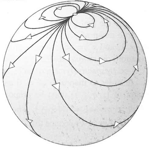

However, gravity in the spherical world has major problems: unlike charges, there are no negative mass objects. Unless there’s no matter, total mass can never be 0. Note we’re discussing this problem under the classical mechanics framework. Under general relativity, gravity is no longer a vector and Gauss’s flux law doesn’t apply, so these problems no longer exist. Matter can exist in de Sitter universes.

Derivation of Spherical Geometry Formulas

To quantitatively calculate gravitational decay, let’s derive expressions for circumference, area, etc. in spherical and hyperbolic geometries. Hint: If you’re not interested in formula derivations, you can skip this section quickly.

Derivation of Spherical Circle Circumference Formula

This is a high school level problem. Given a circle’s radius $r$, the corresponding central angle of this arc on the sphere in 3D space is r (this is the definition of radians). To find the circle’s circumference, we need to know its radius in 3D space, which is the sine of the central angle, i.e., $\sin(r)$. Thus we obtain the spherical circle circumference formula: $$c(r)=2\pi \sin(r)$$

From this formula we can see:

1. Spherical circle circumference first increases then decreases with radius. When radius is $\pi$, the circle’s circumference becomes 0 - at this point the circle has shrunk to a point on the opposite side of the center.
2. When the radius is small, $\sin(r)\approx r$, and the spherical circle circumference formula is the same as the planar circle circumference formula.

Derivation of Spherical Circle Area Formula

Area calculation is normally quite complex, but since we already know the spherical circle circumference formula, we can calculate area through integration: divide the solid circle into many concentric small rings, and the sum of these rings’ circumferences times their thickness gives the total circle area. Let’s verify by deriving the normal Euclidean circle area:
$$S(r)=\int_0^r2\pi u \mathrm{d} u=\pi r^2$$

Similarly, we can directly integrate the spherical circle circumference expression with respect to radius to get spherical circle area:
$$S(r)=\int_0^r2\pi \sin(u) \mathrm{d} u=2\pi(1-\cos(r))$$

Note $S(\pi)=4\pi$, at which point the spherical circle covers the entire sphere, exactly the total spherical surface area.

The Hyperboloid Model

The distance formula in hyperbolic space using the Poincaré disk is somewhat complex, so let’s switch to using the hyperboloid model in Minkowski space to calculate circumferences. If readers are unclear about Minkowski space and hyperbolic angles, please read the article “Geometry of Minkowski Space and Constant Curvature Spaces“.

Derivation of Hyperbolic Circle Circumference Formula

In the hyperboloid model, the hyperbolic world is the following two-sheet hyperboloid in 3D Minkowski space:
$$x^2+y^2-z^2=-1$$

Let’s place the circle’s center on the $z$ axis, at point $(0,0,1)$. Circles centered here can be obtained by intersecting the hyperboloid with planes parallel to the $xy$ plane. From the figure below, we can see that the circle’s radius actually corresponds to the arc length $r$ of a hyperbola segment, which can be measured by the hyperbolic angle $r$. How do we calculate this circle’s circumference under the Minkowski metric? The Pythagorean theorem in Minkowski space is $ds^2=dx^2+dy^2-dz^2$. Since the entire circle is perpendicular to the $w$ axis, $dw$ is 0, so for this circle, it’s completely calculated using the normal distance $ds^2=dx^2+dy^2$, i.e., using the formula $2\pi R$, except here the radius $R$ corresponds to the radius in 3D space. Similar to trigonometric functions in circles, given a hyperbolic angle, we use hyperbolic cosine for horizontal coordinates and hyperbolic sine for vertical coordinates. But the hyperbola here is rotated 90 degrees from when defining hyperbolic functions, so for example the horizontal coordinate in the figure is the hyperbolic sine of the circle’s radius $\sinh(r)$. Thus we finally obtain the hyperbolic space circle circumference formula as $2\pi \sinh(r)$. Compare with the spherical circle circumference formula: $2\pi \sin(r)$ - their difference is just in their respective trigonometric functions. When $r$ is small, both $\sin(r)$ and $\sinh(r)$ approach $r$, both matching the Euclidean circle circumference formula.

Derivation of Hyperbolic Circle Area Formula

With circumference calculated, area can naturally be quickly obtained through integration:
$$S(r)=\int_0^r2\pi \sinh(u) \mathrm{d} u=2\pi(\cosh(r)-1)$$

When $r$ is small, does this circle area formula match $\pi r^2$? The answer is yes: taking the first two terms of the Taylor expansion of $\cosh(r)$, we get $\cosh(r)=1+r^2/2$, which can be verified.

Derivation of Hyperbolic Equidistant Curve Distance Formula

Later, when calculating half-plane planet gravity, we’ll encounter the problem of comparing lengths of lines and equidistant curves. As mentioned before, equidistant curves parallel to lines are longer than the lines. How much longer exactly? Both lines extend infinitely, so we must specify a method for comparing lengths, otherwise discussing which is longer becomes meaningless. Since the distance between them is constant everywhere, the most intuitive approach is to draw many perpendicular segments of equal length between the two lines. It can be verified that the ratio of line segment lengths between two perpendicular segments is independent of the choice of perpendicular segments. Although the total lengths are infinite, we can know how much longer the equidistant curve is through this ratio.

For an equidistant curve at distance $r$ from a line, how many times longer is it than the line? For such seemingly intractable geometric problems, we can start with spherical space. On a sphere, the Tropic of Cancer and the equator are like equidistant curves and lines. It’s easy to verify that the ratio of arc lengths between perpendicular segments is just the ratio of the two circles’ circumferences. Setting the sphere radius as 1, the radius of an equidistant circle at spherical distance r is $\cos(r)$, and the circumference ratio is the radius ratio. Therefore, we obtain that an equidistant curve at distance $r$ from a line on a sphere has length $\cos(r)$ times the line.

Now for the hyperboloid. Similar to the sphere, equidistant curves and lines in hyperbolic space can be obtained by intersecting the hyperboloid with a set of parallel planes, one passing through the origin and one not. Algebraically, it can be proven that both intersections are hyperbolas with similar shapes. Informally speaking, we can calculate the hyperbola length ratio based on the “radius” ratio. This isn’t geometrically obvious, but can be verified through algebraic calculation. We can see that given hyperbolic distance $r$, the radius here is $\cosh(r)$, which is the length ratio of equidistant curve to line.

Gravitational Distribution of Symmetric Planets

With the geometric formulas derived above, we can calculate the gravity of various shaped planets in a 2D universe.

External Gravitational Distribution of Circular Planets

This case is the simplest. The derivation process is the same as in flat space, just note that the circle circumference formula $c(r)$ is no longer $2\pi r$.

Draw two concentric circles with radii $r_1$ and $r_2$. By symmetry, all electric field lines emitted by charge $q$ pass through both concentric circles. This flux can be obtained by multiplying field strength by circumference, so we have $c(r_1) E(r_1)=c(r_2) E(r_2)$, i.e., $c(r) E(r)$ is constant, yielding that $E(r)$ is inversely proportional to circumference.

In flat space, $c(r)=2\pi r$, so field strength decays inversely with distance, while in hyperbolic space $c(r)=2\pi \sinh(r)$, hyperbolic sine grows exponentially with distance, so $E(r)$ also decays exponentially with distance. We’ve proven through calculation our earlier conjecture about the hyperbolic universe: all interactions decay very quickly.

Internal Gravitational Distribution of Circular Planets

If we live on a spherical planet in a hyperbolic world and dig a vertical shaft toward the planet’s center, how would the gravity experienced by people in the shaft change? This problem is handled similarly to flat space. Let the planet’s radius be $R$ and the distance from the shaft bottom to the planet center be $r$. Then people at the shaft bottom only feel gravity from the sphere of radius $r$ beneath their feet. Why? After removing the sphere beneath their feet, people at the shaft bottom are on the inner wall of a shell planet, thus experiencing no gravity.

Assuming the planet has constant density, we can calculate the mass of the portion beneath through circle area, thus calculating gravity. Let the area of a circle with radius $r$ in hyperbolic space be $s(r)$. Then gravity in the shaft is ${s(r)c(R)\over s(R)c(r)}$ times surface gravity. Substituting the specific formulas derived earlier:
$${(\cosh(r)-1)\sinh(R)\over(\cosh(R)-1)\sinh(r)}$$

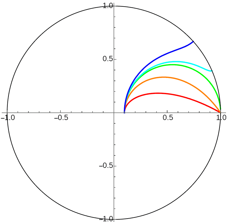
Now we can draw the complete gravitational distribution of a 2D circular planet in hyperbolic space: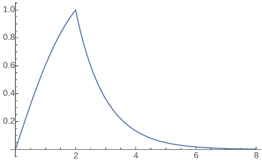

If the planet radius is much smaller than the space curvature radius, the gravitational distribution degenerates to the flat space case: linear gravity inside the planet, inverse decay gravity outside.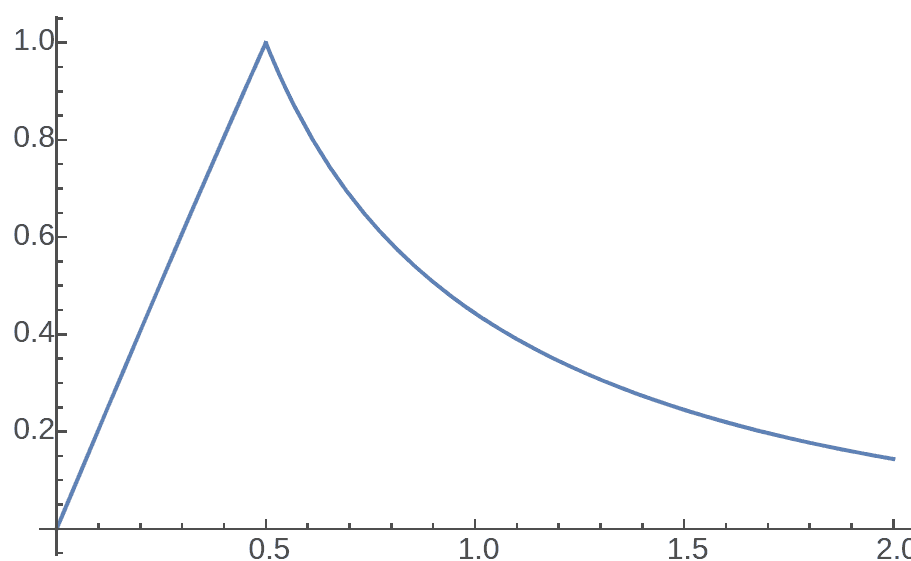

Gravitational Distribution of Horocycle Planets

Finally, let’s calculate the gravity of infinitely large planets! The previous calculations used figure symmetry, so following the pattern of surrounding point charges with circles, we need to construct a series of equidistant curves of horocycles. As long as we understand the circumference ratios between these equidistant curves, we can know how the electric field is diluted. Obviously, the equidistant curves of circles should be concentric circles. As the name suggests, horocycles are a limit of ordinary circles. Therefore, when the planet radius is very large, its field strength approaches that of an infinitely large horocycle planet: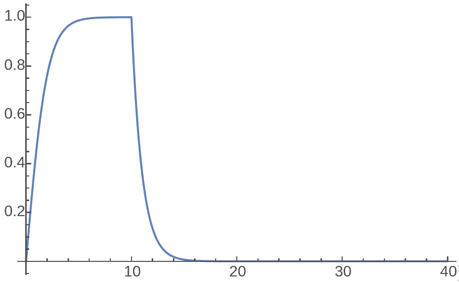

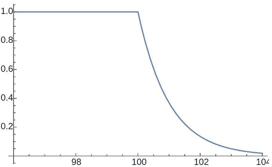
For a true horocycle planet, by taking limits it’s not hard to find that the field strength outside the planet has a standard exponential relationship with distance, while gravity inside the planet is constant! Of course, for such a planet’s gravity to be finite at the surface, it needs density approaching zero - that is, only a horocycle planet made of almost infinitely “light” ultra-low density material can exist with finite surface gravity.

External Gravitational Distribution of Half-Plane Planets

After horocycles come equidistant curves and half-plane planets. Let’s first look at the simpler half-plane planet. Half-plane planets are infinitely large and can’t be obtained by continuing to increase circle radius, because continuing to increase a horocycle’s radius still yields a horocycle, i.e., the infinitely many concentric horocycles drawn earlier. Therefore, we must recalculate half-plane planet gravity. By symmetry, perpendicular to the gravity direction are rings of equidistant curves. Although equidistant curves have infinite length, due to the geometric effect mentioned above, field strength will indeed be exponentially diluted by $\cosh(h)$ as distance $h$ increases. Imagine the entire universe split in half - one half a solid planet, one half vacuum universe. However, due to the special nature of hyperbolic space, after moving slightly away from the planet, its gravity will decay exponentially. A bit farther and this planet will quickly disappear from view. The remaining half of the vacuum universe can completely accommodate infinitely many half-plane planets of the same size, each planet being half the universe!

Internal Gravitational Distribution of Half-Plane Planets

Next, let’s calculate the gravitational field inside half-plane planets: i.e., digging a shaft of depth $d$, the gravity magnitude at the bottom. By symmetry, we similarly create equidistant curves parallel to the ground. From the figure below, we can see that gravity inside half-plane planets is special in that in a certain sense, the land beneath your feet is more than the entire planet: gravity felt in a shaft at certain depth is equivalent to the total gravity of the portion below the equidistant curve at your feet (yellow + red), but this portion of the planet not only contains another entire half-plane planet’s worth of matter (red), but also includes the yellow region’s matter. Relative to the surface, gravity becomes stronger, and the yellow portion’s gravitational resultant points upward. This is a big problem, because if surface gravity is a finite downward value, then after the shaft exceeds a certain depth, gravity will decay to zero. Then going deeper, people don’t feel they’re at the bottom of a well - they instead feel they’re at the “top”, and if not careful, they risk falling upward! There’s another effect: if you fly maintaining altitude at sufficient depth below the planet’s surface, you need to provide centripetal force pointing toward the sky! Under certain conditions, this centripetal force can be provided by gravity! But later calculations show that gravity for such infinite planets is difficult to obtain a reasonable finite value through limits, so I’m inclined to think solid half-plane planets can’t be reasonably constructed, and those bizarre events of “falling up” from well bottoms actually have no chance of occurring.

If we relax some conditions, we can still obtain meaningful infinite planets. For example, an infinitely long shell-like planet shaped like a belt, centered on a line with two equidistant curves as surfaces, dividing the universe in half. This infinite celestial body has finite gravity.

3D Hyperbolic Universe

We’ve been discussing 2D universes, quite different from our universe. If the universe is 3D, the method for calculating planetary gravity is actually similar, except finding circle circumference becomes finding surface area, finding area becomes finding volume, finding the length ratio of equidistant curves to lines becomes finding the area ratio of equidistant surfaces to geodesic surfaces (the analogue of planes)…

Here are the corresponding geometric formulas:

• Surface area of sphere with radius $r$: $4\pi \sinh^2(r)$
• Volume of sphere with radius $r$: $\pi(\sinh(2r)-2r)$
• Area ratio of equidistant surface to geodesic surface separated by distance $d$: $\cosh^2(d)$

The gravitational decay properties of planets in 3D and 2D hyperbolic universes are also similar. Spherical planets have external gravity decaying as inverse hyperbolic sine squared, which is no different from exponential decay since $\sinh^2(x)$ growth rate quickly approaches $\exp(2x)/4$. Horocycle planets similarly have constant internal gravity… I won’t draw these gravity change curves here. Below are the expressions for internal and external gravitational fields of spheres and horocycles:

• Field strength at distance r from center of planet with radius $R$:$$r<R:k{(\sinh(2r)-2r)\sinh^2(R)\over(\sinh(2R)-2R)\sinh^2(r)}$$$$r>R:k{\sinh^2(R)\over\sinh^2(r)}$$
• Field strength at distance r from horocycle surface:Interior: $k$
  Exterior: $k\exp(-2r)$

What’s the intuitive experience of living in these hyperbolic worlds? There’s already a game abroad: Hyperbolica, which I’ve introduced before. This game world is a half-space planet. The author didn’t consider Gauss’s theorem and set gravity to be constant everywhere, directly avoiding the infinite gravity paradox of infinitely large volume planets pointed out earlier.

Geometry of Horocycle Planets

There are actually some interesting aspects about horocycle-shaped planets:

1. What are the geodesics on this horocycle planet? Imagine the equator and small circles on a sphere - obviously the equator is “straight” with no curvature, while small circles have curvature. Horocycle planets are also like “small spheres” in the hyperbolic universe, with surfaces that have constant curvature. Horocycles are limits of ordinary spheres, so the straightest lines (geodesics) on them are naturally great circles. Since the horocycle’s center is at infinity, these great circles are all horocycles going to infinity.
2. Following spherical triangles and spherical circles, we can also define horocycle spherical circles on the surface of horocycle planets. What’s the relationship between circumference and radius? Calculations reveal the circumference formula is surprisingly just $2\pi r$, completely the same as the planar case. What’s going on? First, the radius $r$ of a horocycle spherical circle is an arc length on a horocycle. The radius of this circle in true hyperbolic space should be half of a chord inside the horocycle, i.e., $r’$ in the figure. We know circumference in hyperbolic space has an exponential relationship with radius, i.e., when $r’$ is short, the circle’s circumference can still be very long. Similarly, when the chord is short, the corresponding horocycle arc can also be very long. After these two exponential relationships cancel out, on the horocycle surface it actually returns to the same situation as a flat 2D plane.

Actually, the metric on a horocycle surface is completely equivalent to a 2D Euclidean plane. This planet’s world map can be completely drawn on a plane with no distortion anywhere! Unfortunately, this zero-curvature world map can’t fit well into the negative-curvature hyperbolic universe where the planet resides…

Stability of Celestial Motion

We’ve already witnessed the stability issues of star-planet system orbits in universes of different dimensions and even different norm spaces. In hyperbolic space, gravitational decay changes from polynomial to exponential, an even more dramatic change. Does this mean there are no stable planetary orbits? Let’s calculate and simulate. The standard approach is to calculate the “Christoffel symbols” that reflect the difference between curved and flat space derivative operators, to correct for geodesic deviation caused by curvature. These tedious differential geometry calculations give me a headache - I almost didn’t want to write this. Later I thought of a method to solve directly on the hyperboloid model, which should be more interesting and can bypass differential geometry - imagine how to calculate the motion of a point mass fixed on a sphere: when the point mass experiences no force, its trajectory is a great circle, because as long as it moves on the sphere, it must experience a centripetal force on the sphere’s normal proportional to velocity squared. This force constrains it to the sphere. We can similarly calculate a force proportional to velocity squared for a point mass moving on a hyperboloid to keep it fixed on the hyperboloid. The gravity model is even simpler: first convert distance in the hyperboloid model to hyperbolic distance within the hyperboloid using inverse hyperbolic functions, then calculate gravity magnitude using previous formulas. The direction of gravity is the tangent vector of the line connecting that point on the hyperboloid to the origin. The point mass experiences both gravity tangent to the hyperboloid and constraint force on the normal. This allows us to write kinematic equations for numerical solution. Note these vectors are all calculated in a 3D Cartesian coordinate system. Adding the hyperboloid equation constraint actually gives differential equations with two variables. If I haven’t miscalculated, it should match the “Christoffel symbol” calculation results.

Click here to show/hide all my calculation process

Consider the unit two-sheet hyperboloid $z^2=1+x^2+y^2$ as the geometric model of hyperbolic space. Let the central body be at $(0,0,1)$ and the planet at $(x,y,\sqrt{1+x^2+y^2})$. I’ll list some equations - if there are errors, please point them out:

• The direction of gravity on the planet is the tangent to the geodesic connecting $(0,0,1)$ to that point on the hyperboloid at the planet’s location. The geodesic is cut by a plane through the origin, so this tangent is in the plane determined by the origin, planet, and sun. Based on this geometric relationship, we can derive that the unit vector of gravity direction on the planet is $\tau(x,y)=(k x, k y, \sqrt{x^2+y^2})$, where $k=\sqrt{1+{1\over x^2+y^2}}$;
• If the planet is at $(x,y,\sqrt{1+x^2+y^2})$, its distance from the central body within hyperbolic space is $d(x,y)=\mathrm{arcsinh}(\sqrt{x^2+y^2})$
• Since I want the differential equations to only contain letters $x$, $y$ and time $t$, I need to express the planet’s velocity vector magnitude using $\dot{x}$ and $\dot{y}$. Note the planet moves on the hyperboloid, so the z-axis also has a velocity component. Intuitively, $(\dot{x},\dot{y})$ is just the projection of the 3D velocity onto the xy plane. We can decompose the 3D velocity into components parallel and perpendicular to the line connecting to the central body. The magnification factors for projecting these two parts onto the xy plane are $\sqrt{1+x^2+y^2}$ and $1$ respectively. Based on this relationship, we can write the expression for the 3D velocity vector magnitude: $$v(x,y,\dot x,\dot y)=\sqrt{\frac{\left(x^2+1\right)\dot y^2-2x\dot xy\dot y+\dot x^2\left(y^2+1\right)}{x^2+y^2+1}}$$
• The constraint force direction on the planet is normal, i.e., from origin pointing to the planet. The acceleration in this part is velocity squared divided by radius 1, i.e., $(x,y,\sqrt{1+x^2+y^2}) v^2(x,y,\dot x,\dot y)$.
• Let dimension be $n$, with gravitational coefficient $G$ absorbing the planet’s mass. Then the planet’s acceleration is $-{\tau(x,y) G \over \sinh^{n-1}(d(x,y))}$
• Writing out the $x$ and $y$ components of the acceleration expression gives the final differential equations: $$\ddot x=v^2(x,y,\dot x,\dot y)x-{G\tau_x(x,y) \over \sinh^{n-1}(d(x,y))}$$$$\ddot y=v^2(x,y,\dot x,\dot y)y-{G\tau_y(x,y) \over \sinh^{n-1}(d(x,y))}$$

Fortunately, all these calculated things can be directly thrown to Mathematica for computation. The final conclusion is consistent with previously discussed flat space and even p-norm spaces: planetary orbits in 3D space are not only stable but also closed orbits without any precession - this result is quite beautiful. In spaces with dimension less than three, planetary orbits are petal-shaped with precession, while in dimensions greater than three, orbits are unstable. Why are cube-inverse orbits in 4D space unstable while exponentially decaying gravitational orbits in hyperbolic space are still stable? I think space also increases exponentially, providing a kind of negative feedback effect to some degree. If you look carefully at the hidden formula derivation above, you’ll find that exponential hyperbolic sines and inverse hyperbolic sines cancel out, with no exponential terms in $x$ and $y$ in the equations. (Assuming I haven’t miscalculated!)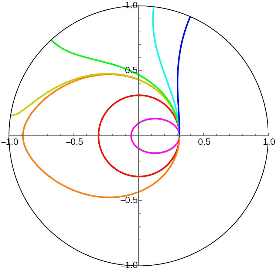

2D hyperbolic worlds produce petal-shaped precession like flat space. When initial velocity exceeds a certain range, Mathematica reports convergence errors, so I can’t verify whether there are escape orbits. But through energy calculations, we can verify that the energy needed to move a point mass from finite distance to infinity is finite (the improper integral $\int^{+\infty}_r \mathrm{d}x/\sinh(x)$ converges), so there won’t be no escape velocity like in 2D flat space.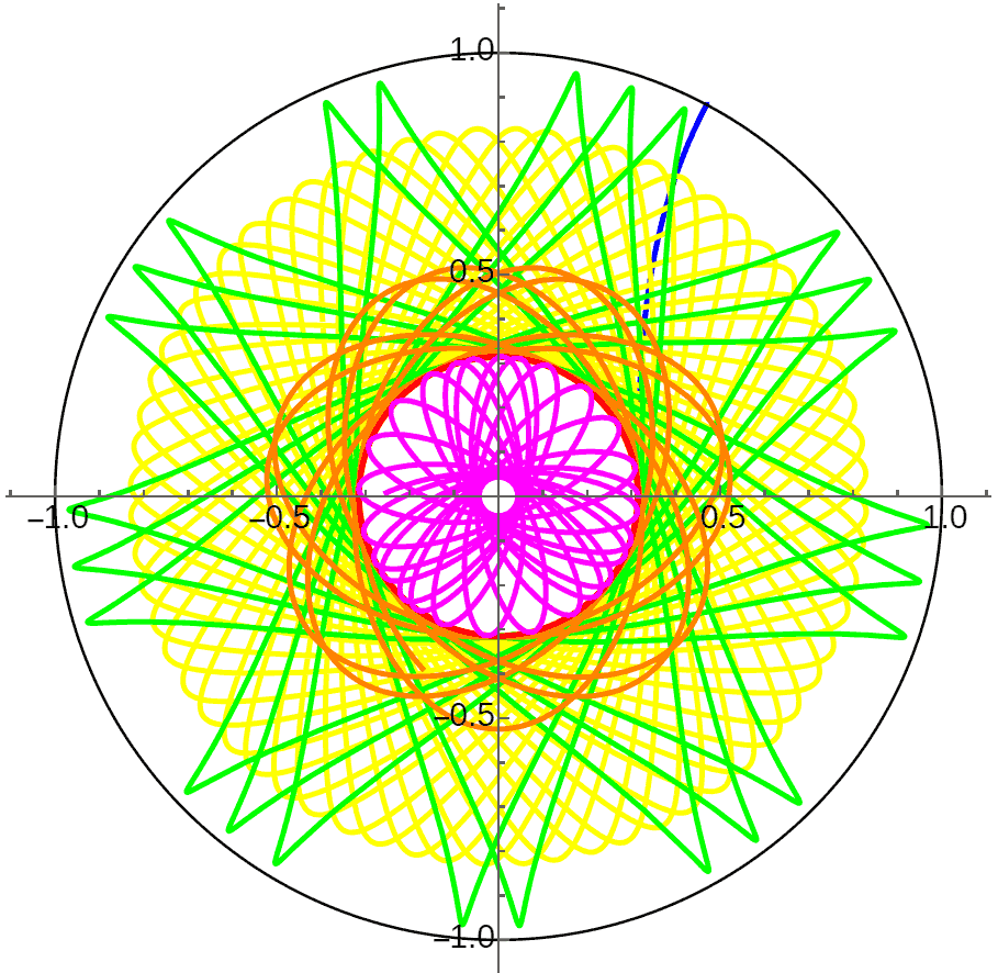

4D hyperbolic space orbits remain unstable: the red and blue orbits have initial velocity relative errors of only one part in ten billion, yet after just two orbits around the celestial body they have completely different fates: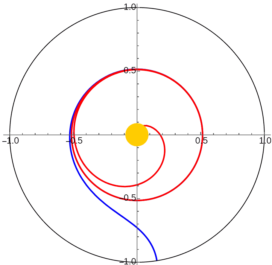

Finally, there’s something strange: if celestial bodies aren’t connected by gravity but by springs (i.e., central force proportional to distance), planetary orbits in flat space are closed ellipses, but as hyperbolic space curvature increases, elliptical orbits will precess more and more, becoming petal-shaped. But why don’t planets under inverse square gravity have any precession at all? Perhaps my calculations are wrong, or this is indeed the fact with some deep theory behind it? I hope experts can answer…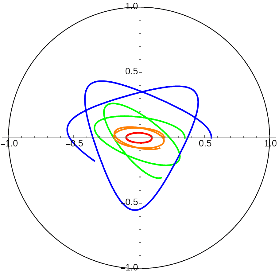

Central Body at Infinity

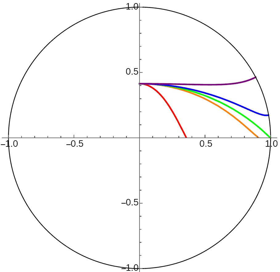
Finally, let’s tackle calculating planetary stability when the central body is at infinity (same as external gravitational distribution of horocycle planets). Note that planetary orbits are no longer periodic motion, because horocycles have infinite radius and circumference. How to calculate gravity? First, we must clarify that we can’t calculate the distance from planet to infinity, but we can find the difference in distance from planet and a reference point (like the origin) to the central body through the exponential decay law of gravity with distance to calculate gravity ratio. Second is calculating gravity direction: it’s along the tangent at the planet to the geodesic passing through the point at infinity and the planet. How to calculate specifically? We can still complete all calculations in the hyperboloid model! Calculation process also hidden here, click this link to expand

Still consider the unit two-sheet hyperboloid model $z^2=1+x^2+y^2$. Assume the central body is at $(+\infty,0,+\infty)$ and the planet at $(x,y,\sqrt{1+x^2+y^2})$. Then:

• The previous article mentioned horocycles are obtained by intersecting the hyperboloid with planes parallel to any asymptotic line of the hyperboloid. Based on this, by observation we can directly write the plane equations of all horocycles passing through $(+\infty,0,+\infty)$ as $z=x+k$. Substituting planet coordinates, we can find the plane equation of the horocycle containing the planet has $k=\sqrt{1+x^2+y^2}-x$;
• To calculate gravity magnitude, next find the distance between this horocycle and the horocycle passing through $(0,0,1)$ (i.e., the difference of two infinite radii). Since the geodesic connecting $(0,0,1)$ and $(+\infty,0,+\infty)$ is a horocycle radius direction that’s easiest for calculating distance, we need to find the intersection coordinates of the planet’s horocycle with this geodesic. It can be solved by simultaneously solving the three equations of hyperboloid, horocycle plane, and xz coordinate plane: $({1-k^2\over 2k},0,{1+k^2\over 2k})$. Obviously the distance between these two horocycles is the distance from this point to $(0,0,1)$, i.e., a hyperbolic arc. We can find the distance through standard inverse hyperbolic function definition: $d=\mathrm{arcsinh}({1-k^2\over 2k})$. Then according to the gravity formula above, the planet experiences gravity magnitude $G\exp(2d)$.
• To calculate gravity direction, first find the equation of the geodesic connecting the planet to the infinitely distant central body. By observation, all geodesics passing through the infinitely distant central body are obtained by intersecting the paraboloid with plane $k_1(z-x)=k_2 y$. This can be verified by substituting the point at infinity $\lim_{x\to \infty}(x,0,\sqrt{1+x^2+0^2})$. Now substitute planet coordinates to get $k_1(\sqrt{1+x^2+y^2}-x)=y k_2$. Note we don’t treat $k_1/k_2$ or $k_2/k_1$ as one parameter because we need to consider cases where $k_2$ or $k_1$ is zero.
• Next solve for tangent direction. Eliminate $z$ by combining plane and paraboloid equations, treat $y$ as function $y(x)$, and through implicit differentiation technique, we can calculate that this geodesic’s y-direction derivative with respect to x-direction satisfies: $$k_1({x+y y’\over z}-1)=k_2 y’$$ Solving for $y’=\mathrm{d}y/\mathrm{d}x$ from the above equation gives the ratio of tangent’s y and x components: $$(y^2+z(x-z))\mathrm{d}y=-y (x-z)\mathrm{d}x$$
  We can assume unit tangent vector $\tau=(a (y^2+z(x-z)),-a y (x-z),b)$, and solve for coefficients $a$ and $b$ by combining the conditions that unit vector length is 1 and tangent vector is always perpendicular to planet’s position vector: $$\tau.(x,y,z)=0$$ $$|\tau|^2=1$$
• Now we can finally write the planet’s equations of motion. Note acceleration includes not only gravity but also the previously derived surface constraint force term:
  $$\ddot x=v^2(x,y,\dot x,\dot y)x+G\tau_x(x,y) \exp(2d)$$$$\ddot y=v^2(x,y,\dot x,\dot y)y+G\tau_y(x,y) \exp(2d)$$

From the calculation results, we find that since horocycle circumference is infinite, planets either continuously approach or recede from the central body, because planets can never reach the “perihelion” or “aphelion” located at infinity. So this is actually similar to the unstable orbits with cube-inverse in 4D space. Note that although the red, orange, and green orbits in the figure appear to all approach the infinitely distant central body in the Poincaré disk model, actually the green orbit is a horocycle - the planet maintains constant distance from the infinitely distant central body doing “uniform horocycle motion”, while the red and orange orbits are truly continuously falling toward the horocycle center due to insufficient initial velocity. Planets can reach the infinitely distant central body in finite time along these orbits with crazy acceleration! Although we’re only discussing Newtonian mechanics in hyperbolic space here, this is very much like objects falling into black holes and reaching the singularity in finite time.

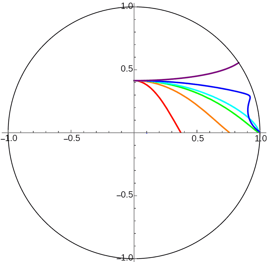
Initially I thought all planetary orbits in the gravitational field of infinitely distant central bodies followed this pattern. Later, when trying to calculate theoretical orbits of planets inside horocycle planets, I found strange results and realized something was wrong: gravity formulas in different dimensions are all exponential functions of distance, just with different coefficients - the gravitational expression in $n$-dimensional space is $\exp(nd)$. I initially mistakenly thought this coefficient didn’t affect orbit shape, but this coefficient actually comes out as a power $(\exp(d))^n$, which does affect orbit shape and stability. Calculation results for 2D hyperbolic world orbits revealed planetary motion is actually periodic! I think the main difference from the 3D case is that 2D space orbits have precession, causing “perihelion” and “aphelion” to no longer be at opposite ends of circular orbits. When the circle approaches infinity becoming a horocycle, both “perihelion” and “aphelion” will be at finite positions, with infinitely many “perihelions” and “aphelions” appearing on the horocycle! We can see the period of “perihelion” and “aphelion” appearance on the horocycle decreases as initial velocity increases, with a limiting period (corresponding to orbits just below escape velocity, like the purple orbit in the figure).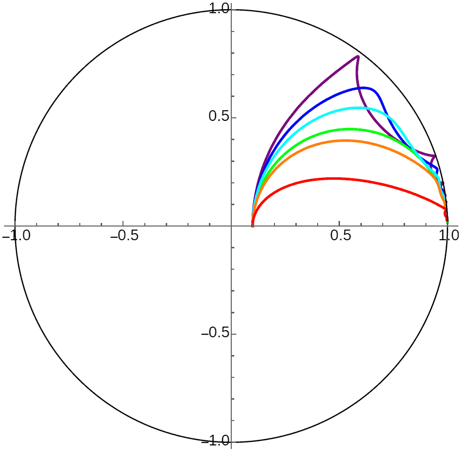

You might not see the periodicity in the orbits above, so here’s an animation of ideal rotation along a horocycle:

If space dimension is four, orbits become unstable. The difference from 3D is that orbit divergence and convergence are faster, more sensitive to initial velocity precision for horocycle orbits. I won’t show figures here.

Planets Inside Horocycle Planets

There’s another case that only makes mathematical sense: planets inside horocycle planets experiencing constant magnitude gravity pointing toward the sphere center. Although planets can’t actually orbit inside another celestial body, we can still explore orbital stability: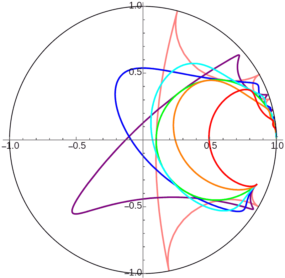

It’s similar to 2D horocycle planet external orbits, but since gravity is constant without decay, planetary escape velocity is infinite. When velocity approaches infinity (pink orbit in figure), its trajectory approaches free motion geodesics. At great distances, the geodesic direction becomes opposite to the direction pointing to the horocycle center. Gravity can continuously do negative work until making the planet turn around and fall back! Note that orbits with initial velocity greater than horocycle orbit always have “perihelion” tangent to the horocycle orbit, while orbits with initial velocity less than horocycle orbit have “aphelion” all tangent to the horocycle orbit.

Planets Orbiting Shell Infinite Plane Planets

Finally, we can calculate orbits in the external gravitational field of shell infinite plane (geodesic surface) planets. (Note: such infinite planets have the same external gravity as half-space planets, but finite internal gravity, so they can exist.) The “circular” orbit of planets orbiting them has now become equidistant curves. If planetary initial velocity changes slightly, what’s the orbital stability in different dimensions? The calculation is actually somewhat less than for horocycles, but calculation process is also hidden here, click this link to expand

Still consider the unit two-sheet hyperboloid model $z^2=1+x^2+y^2$. The infinite planet surface is the geodesic where the hyperboloid intersects the xz plane. Let the half with $x>0$ be the sky where the planet is located, and the other half be the ground. The planet is at $(x,y,\sqrt{1+x^2+y^2})$. Then:

• To find the planet’s height above ground, we need to create an equidistant curve through the planet parallel to the ground. The previous article mentioned equidistant curves are obtained by intersecting the hyperboloid with planes not passing through the origin and parallel to the plane containing its axis. Therefore, the plane containing the equidistant curve is the plane perpendicular to the y-axis with intercept equal to the planet’s y-coordinate value. Obviously the planet’s height is $d=\mathrm{arcsinh}(y)$.
• To find gravity direction $\tau$, we need to create a geodesic through the planet perpendicular to the ground. Obviously the equation of the plane containing this geodesic can be set as $k_1 z=k_2 x$. Following the previous horocycle approach, after combining with the hyperboloid equation and implicit differentiation, we get the ratio of gravity direction’s x and y components: $$k_1 {x+y y’\over z}=k_2$$ Substituting planet coordinates to replace $k_1,k_2$ and simplifying: $$xy \mathrm{d}y = (1+y^2) \mathrm{d}x$$ Finally, solving for all component values through the conditions that this direction is a unit tangent and orthogonal to the position vector, the first two components we care about are: $$\tau_x=-{xy\over\sqrt{1+y^2}}$$$$\tau_y=-\sqrt{1+y^2}$$
• Finally adding curvature correction terms to write the kinematic equations:
  $$\ddot x=v^2(x,y,\dot x,\dot y)x+{G\tau_x(x,y)\over \cosh^2(d)}$$$$\ddot y=v^2(x,y,\dot x,\dot y)y+{G\tau_y(x,y)\over \cosh^2(d)}$$

Since the ground no longer has curvature, all planets with initial velocity less than first cosmic velocity will crash. Those equal to first cosmic velocity move along equidistant curves maintaining constant height. Those greater than first cosmic velocity will escape if dimension is three. In 2D there are two cases - it also has a second cosmic velocity. Planets with velocity greater than first cosmic velocity but less than second cosmic velocity will rise to a certain height (reaching “aphelion”) then descend, but won’t crash to the ground. Only those greater than second cosmic velocity will completely escape.

Don’t think from the figures above that 2D space planets with velocity between first and second cosmic velocities will climb once then slowly descend approaching a fixed height. Actually, their orbits will rise again at great distances - they’re also periodic! This is easy to understand, since viewing a shell infinite plane planet from far away is the same as viewing a point celestial body at infinity. But unlike the infinitely distant central body case, planets above infinite plane planets with velocity less than first cosmic velocity won’t have periods - they definitely can’t escape the fate of crashing to the ground. The figure below shows an animation of the Poincaré disk shifted right to see distant orbits clearly:

Speculation: Hyperbolic World with Relativity

Previous articles have introduced de Sitter/anti-de Sitter spacetime, representing the spacetime geometry of spherical/hyperbolic worlds ignoring gravity. After considering relativity, object motion no longer has extra tidal forces, because we’ve already analyzed the isotropy of this space - no special reference frame can be found. It’s worth noting that parallel timelike geodesics in this space itself tend to approach each other, so regardless of whether objects move relative to the observer, objects internally will bear a constant positive pressure to maintain their volume and not collapse to a point.

Finally, I have some wild thoughts (forgive me for not being familiar with general relativity content, corrections from professionals welcome): Can general relativity framework allow infinitely large planets like horocycles and half-planes to exist? I’m not familiar with specific calculations in general relativity, but I imagine perhaps there’s a black hole singularity at infinity with its event horizon being a horocycle? Or due to infinite distance, the singularity can’t actually be reached - perhaps there could even be a naked singularity at infinity while satisfying the cosmic censorship hypothesis? Whether these descriptions are correct is questionable, because if anti-de Sitter space has a black hole at infinity, then it should no longer be constant curvature anti-de Sitter space. Unlike Schwarzschild black holes whose spacetime is asymptotically flat, a black hole at infinity makes “asymptotically anti-de Sitter” lose meaning…