Introduction to Type Theory and Machine Proof
The previous article introduced propositional logic, first-order logic, and ZFC set theory. This article examines a new approach that claims to replace set theory’s position in mathematics — type theory. In fact, it has been widely used in machine proofs, most famously in the proof of the Four Color Theorem. Additionally, it is very similar to programming code. When type theory is modified into homotopy type theory, it can handle many problems in topology more “directly” than set theory.
Motivation for Type Theory
The concept of “type” is widely used in programming languages, specifically for type checking before compilation. For example, consider this C code:
int i = 0;       // Define integer variable i and set it to 0
string j ="oma"; // Define string variable j and set it to "oma"
int k = i * j;   // Define integer variable k and set it to i * j
This will cause a compilation error because the program declares i as an integer type variable and j as a string type variable, and they cannot be multiplied. In other words, multiplication is a function that takes two numbers as input parameters and returns a number as output—the types of i and j clearly don’t match this. From this example, we can see that type checking is essentially the compiler helping us check for obvious low-level errors that would lead to meaningless operations like multiplying numbers by strings. Although checking the type of an expression is also mechanized (can be defined as a formal system), this seems to have nothing to do with mathematical logic. How can it be used to construct axiomatic systems? yugu233 made a video “On the Similarity Between Programmers and Mathematicians [Mathematical Map]” that explains the connection between types and proofs in a very accessible and vivid way.
Optional reading aside:
I wonder if any readers are familiar with TypeScript (JavaScript with type checking). Its type inference mechanism is very powerful and has reached Turing completeness. Once you know the principles, it’s easy to define natural numbers using pure type inference and perform arithmetic operations. See here for reference. These calculations are completed entirely during compiler type checking. The code contains only a bunch of type declarations, and the compiled executable is empty. Note that this actually has nothing to do with the type theory we’re discussing.
For convenience, we write “variable a has type A” as “a : A”. The reasoning power of type theory mainly comes from facts about functions: Given types A and B, if there exists some function f : A → B, then f can achieve this: given a variable a : A, we can obtain a variable f(a) : B of type B.
Like all formal systems, these functions and variables are just meaningless symbols. If you understand them as computer code, they correspond to variables physically stored in memory and function jump instructions. Now let’s understand them from a completely new perspective: translate “a : A” as “a witnesses that proposition A is true”. That is, translate types as propositions, and translate corresponding variables as evidence that propositions are true. Let’s think about what the following type theory rule represents in this new perspective:
Given “a : A” and “f : A → B”, we can construct “f(a) : B”
This statement says that if propositions A and A → B both hold, then we can deduce that proposition B holds—equivalent to the modus ponens (mp) inference rule in propositional logic! Moreover, the arrow symbol in function types can be interpreted as the logical implication arrow symbol in reasoning! Type theory can actually do much more than this—it can handle not only propositional logic but also first-order logic and higher-order logics with slight modifications. But before that, let’s become more familiar with this formal system. For example, how do we use type theory to prove the following theorem?
If propositions A → B and B → C both hold, then we can deduce that proposition A → C holds
In type theory, a proposition holding means there must exist some value under that type, called the type being inhabited. So we can assume there exist two functions f and g, with f : A → B, g : B → C. As long as we can construct a new function h : A → C, we have proven the original proposition. Obviously, function composition can achieve this—define h(x) = g(f(x)), and it’s easy to verify that h’s type is indeed A → C.
But type theory is a formal system, and we haven’t yet given specific inference rules. Otherwise, we wouldn’t even know if we’re allowed to define h(x) = g(f(x)). Below we’ll briefly introduce the foundation of type theory—λ-calculus.
Untyped Lambda Calculus
There are many kinds of lambda calculus. Untyped λ-calculus is a formal system where everything is a function, similar to set theory’s view that everything is a set. But it’s not based on first-order logic—it has its own syntax for symbol construction and inference rules:
- All valid strings are called “λ-terms”, which can only be constructed using these 3 rules:
- Variables are λ-terms, usually denoted by lowercase letters like x, y, z, a, b, c, f, g, h, etc.
- If x is a variable and M is a λ-term, then (λx.M) is a λ-term. It can be interpreted as the function f(x)=M.
- If M and N are both λ-terms, then (M N) is a λ-term. It can be interpreted as function application M(N).
- λ-terms are just expressions, not assertions or propositions, so there’s another kind of string containing equality that asserts two terms are equal:
- If M and N are both λ-terms, then M = N is a proposition
- λ-terms have three inference rules:
- (α-conversion) The name of the parameter when defining a function doesn’t matter. For example, λx.x and λy.y are the same function. α-conversion states these two are equal: (λx.M) = (λy.M[x/y]), where M[x/y] means replacing free occurrences of x with y. It’s identical to the substitution rule for quantifiers in first-order logic. Example: λx.(λx.x) x = λy.(λx.x) y;
- (β-reduction) Defines function application: (λx.M) N = M[x/N];
- (η-conversion) Clarifies when functions are equal, somewhat like the axiom of extensionality in set theory: λx.f x = f.
- Due to the existence of equality, there are actually two more implicit inference rules:
- (eq1) M = M is an axiom;
- (eq2) If M = N holds, they can be substituted for each other in any λ-term.
A note about parenthesis abbreviations: Without parentheses, the scope of “λx.” extends as far as possible. For example, λx.M N represents (λx.(M N)) not ((λx.M) N).
Why use “λ” to represent functions? Isn’t “f(x)” fine? That’s because when we write “f(x)”, we’ve already implicitly given the function a name “f”. “λ” provides a way to express anonymous functions, now used in many programming languages, though for input convenience they generally use keywords like “function” instead of the symbol “λ”. Note that functions in λ-calculus only have one parameter, but since multivariate functions can be viewed as functions returning functions, this isn’t a problem.
Basic λ-calculus can be used to construct models of boolean values, arithmetic, data structures, and recursion. These are all essentially functions. For example, define TRUE as λx.λy.x, which can be understood as a binary function f(x,y)=x that always returns the first parameter; define FALSE as λx.λy.y, which can be understood as a binary function f(x,y)=y that always returns the second parameter. Readers can verify for themselves using the formal system rules that the functions defined below indeed implement the corresponding boolean logic operations:
AND := λp.λq.p q FALSE
OR := λp.λq.p TRUE q
NOT := λp.p FALSE TRUE
For more on untyped λ-calculus, see Wikipedia.
Typed Lambda Calculus
Untyped λ-calculus sometimes causes problems. For example, β-reduction seems to simplify functions, but sometimes it makes them more complex. Try using β-reduction to simplify the expression “(λx:x x)(λx:x x)” and you’ll find it’s exactly the same before and after simplification. The expression “(λx:(x x) x)(λx:(x x) x)” will “simplify” to “((λx:x x x) (λx:x x x)) (λx:x x x)”, and continuing β-reduction gives “(((λx:x x x) (λx:x x x)) (λx:x x x)) (λx:x x x)”… becoming longer and longer and never stopping. This also means there’s no universal algorithm to determine whether two lambda terms are equal. Type theory uses typed lambda calculus, which prevents this kind of endless self-application loop by introducing types. The rules are roughly as follows:
- Besides the equality symbol “=” that asserts two terms are equal to form propositions, we also introduce the type assertion symbol “:” that asserts the type of values, which also forms propositions
- When defining λ functions, we must specify the parameter type. Types themselves are also terms. For example, (λx:A.M) cannot be written as just (λx.M)
- Introduce two type inference rules:
- (Function construction) If assuming x : A holds allows us to derive y : B in the system, then “(λx:A.y) : A → B” holds;
- (Function application) If f : A → B and x : A hold, then “f x : B” holds. This rule means if function f has type A → B and x has type A, then the result of function application f(x) has type B;
Note: If the function parameter and the applied object have different types, no inference rule can derive the type of that expression—it’s like a compiler detecting a type mismatch error.
Let’s rewrite the proof that A → B and B → C imply A → C:
- f : A → B (given)
- g : B → C (given)
- Introduce assumption x : A
- f x : B (function application 1,3)
- g (f x) : C (function application 2,4)
- (λx:A.g (f x)) : A → C (function construction 3,5)
Note that since the inference rules involve assumptions, each derivation step must specify the current assumption context: the indented 4 and 5 have assumption 3, while the rest have empty assumption contexts. Type theory unifies the concepts of function parameters and assumptions inside functions, equivalent to the role of the deduction metatheorem, so we can also prove that the following type is inhabited, i.e., there exists some value of this type:
? : (A → B) → ((B → C) → (A → C))
The derivation process essentially changes the previously given f and g into assumptions:
- Introduce assumption f : A → B
- Introduce assumption g : B → C
- Introduce assumption x : A
- f x : B (function application 1,3)
- g (f x) : C (function application 2,4)
- (λx:A.g (f x)) : A → C (function construction 3,5)
- (λg:B → C.λx:A.g (f x)) : (B → C) → (A → C) (function construction 2,6)
- (λf:A → B.λg:B → C.λx:A.g (f x)) : (A → B) → ((B → C) → (A → C)) (function construction 1,7)
Does it look a bit complex? If we’re familiar with type theory’s formal system, we can work backwards from the goal to be proven:
- Assumption context: empty
- Evidence to construct: ? : (A → B) → ((B → C) → (A → C))
- Proof goal: ? : (A → B) → ((B → C) → (A → C))
Introduce assumption f : A → B
- Assumption context: f : A → B
- Evidence to construct: λf:A → B.? : (A → B) → ((B → C) → (A → C))
- Proof goal: ? : ((B → C) → (A → C))
Introduce assumption g : B → C
- Assumption context: f : A → B, g : B → C
- Evidence to construct: λf:A → B.λg:B → C.? : (A → B) → ((B → C) → (A → C))
- Proof goal: ? : (A → C)
Introduce assumption x : A
- Assumption context: f : A → B, g : B → C, x : A
- Evidence to construct: λf:A → B.λg:B → C.λx:A.? : (A → B) → ((B → C) → (A → C))
- Proof goal: ? : C
Fill in g (f x) at ?, satisfying the proof goal.
- Proof complete, obtaining the complete evidence (λf:A → B.λg:B → C.λx:A.g (f x)) : (A → B) → ((B → C) → (A → C))
Each time we introduce an assumption, we’re actually constructing a function, but we don’t yet know what value to fill in at “?” in the function body, so we transfer the proof goal to constructing this value. Once all blanks are filled, the entire value is constructed and the proposition is proven. This format is actually the method used by almost all computer proof assistants (like Coq, LEAN, etc.) for writing proofs. Generally, introducing assumptions is written as “intro”, and filling in values is written as “apply” or “exact”. 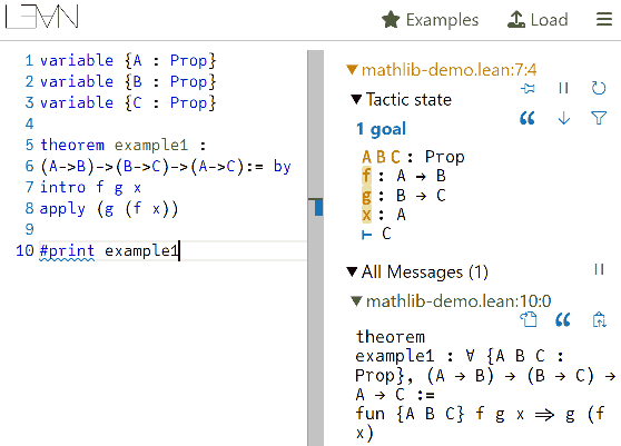
Perhaps you think it’s more satisfying to write the expression all at once and aren’t used to using proof assistants. We’ll see later that as propositions become more complex, proof assistants that help us work backwards from goals become essential. When actually using proof assistants, you only need to keep completing proof goals—details like what the currently constructed evidence looks like are automatically handled and checked by the computer, saving a lot of worry. For example, to prove the proposition (A → B) → ((B → C) → (A → C)), you only need to tell the proof assistant three things:
- Sequentially introduce assumptions f, g, x; (written as intro f g x in LEAN)
- Fill in the value g (f x). (written as apply f (g x) in LEAN)
The rest is automatically completed by the computer for type checking and evidence generation.
Dependent Types, Equality Types, and Definitional Equality
I personally think understanding typed lambda calculus isn’t difficult. The next thing is likely the first “roadblock” on the learning path: dependent types. It arises from this need: since all propositions are types, then “1=1” and “2=2” should certainly be types too. Don’t confuse this with equality in lambda calculus: propositions involving equality are merely types, while the equality defined through (α-conversion) and (β-reduction) is called “definitional equality”—they’re always considered unconditionally equal in the formal system. To distinguish the two, I’ll temporarily write propositional equality as (1 eq 1) and (2 eq 2). In first-order logic, “1=1” and “2=2” are obtained directly from the equality axioms, so type theory also needs to introduce an “equality axiom” rule, directly giving a value of type a eq a:
- For any term $a$, there exists a term “$\mathrm{refl}_a$”, and the type assertion “$\mathrm{refl}_a : a\ \mathrm{eq}\ a$” holds.
Note that type theory is no longer simple lambda calculus, because “atomic terms” in lambda calculus can only be variables or lambda expressions, while type theory also allows constant symbols like refl. This refl is short for reflexivity, representing the reflexive property of equality. Given some type $\mathrm{A}$, to prove that for any $x:\mathrm{A}$, we have “$x\ \mathrm{eq}\ x$” holds, means we need to construct a function that takes any variable $x:\mathrm{A}$ and outputs a variable of type “$x\ \mathrm{eq}\ x$”. This function is easy to construct: it’s $\lambda x : \mathrm{A}. \mathrm{refl}_x$. But what is this function’s type? Imagine if $A$ represents the natural number type. If we input 1, it outputs $\mathrm{refl}_1$, which has type 1 eq 1; if we input 2, it outputs $\mathrm{refl}2$, which has type 2 eq 2. Indeed, the function’s output type depends on the input. Writing it directly as “$\mathrm{A} → x\ \mathrm{eq}\ x$” would be confusing: the x on the right of the arrow appears out of nowhere. So we need to first declare parameter x and introduce the symbol $\prod$ specifically for dependent functions: $\prod{x:A} (x\ \mathrm{eq}\ x)$. In LEAN, dependent function types are represented as: “$(x:\mathrm{A}) → (x\ \mathrm{eq}\ x)$”.
Non-dependent ordinary functions (→) are actually special cases of dependent functions ($\Pi$). We stipulate that the arrow symbol is just shorthand for dependent function $\Pi$, introducing a definitional equality assertion:
$\prod_{x:A}$ B = A → B, if x doesn’t occur freely in B.
For example, the function type (A → B) → ((B → C) → (A → C)) can also be written as $\prod_{f:A → B} \prod_{g:B → C} \prod_{x:A} C$, and further, rewriting f and g’s function types finally becomes: $\prod_{f:\Pi_{x:A} B} \prod_{g:\Pi_{x:B} C} \prod_{x:A} C$.
Why use the product symbol to represent dependent functions is indeed confusing for beginners. While there’s some rationale, it’s mostly a historical artifact not worth dwelling on. When I first encountered this type, I kept getting stuck trying to understand what that product meant. Actually, replacing the product symbol with “$\forall$” makes it easier to understand (that’s how it’s written in LEAN).
Optional reading:
We see that propositional equality types and definitional equality within the system are two different concepts. Their biggest difference is that propositional equality can appear as assumptions in function parameters, while whether two expressions are definitionally equal is fixed and cannot represent the concept of “assuming x and y are definitionally equal” within the system. We could actually forcibly add a rule to make the two kinds of equality no longer essentially different:
- If there exists some term x such that the type assertion “x : a eq b” holds, then the definitional equality assertion “a = b” holds.
However, this is actually unnecessary and shouldn’t be done. Because determining a term’s type is often done automatically by computer systems, and if we equate propositional equality with definitional equality, this would require the computer to have the ability to guess the proof steps for “a = b” during type checking. The most complex and subtle aspect of type theory is in handling equality, which we’ll discuss in detail later.
Universe Types
With dependent function types, we can express not only first-order logic but even second-order logic. For example, “for any proposition A, A → A holds” has quantifiers acting on arbitrary propositions, while in first-order logic quantifiers are only allowed to act on terms (representing sets, natural numbers, etc.), so it’s definitely a proposition in second-order logic. To translate this into type theory, we need to define a function that accepts types, which encounters types of types. Type theory stipulates that the type of all types is called the universe, denoted as “U” (or “Type” in LEAN). But to avoid paradoxes, U’s own type must be a larger universe, denoted as U1, then U1 : U2 : U3 : … forming an infinite hierarchy of type universes. These subscripts can even extend to ordinals, but generally we only need the first level or two.
Besides introducing type-of-type rules, we’ll also update rules to ensure system consistency:
- Only when A’s type is some universe can we introduce assumption x : A.
- If A:Um, B:Un, then $\prod_{x:A}$ B : Umax(m,n), i.e., the universe of a function type is never lower than the universe levels of input and output types.
- If A:Um, B:Un, then A → B : Umax(m,n) (arrow types are special cases of $\Pi$ types)
“For any proposition A, A → A holds” can be translated as this dependent function type being inhabited: $$\prod_{A:\mathrm{U}} A → A$$ Here’s the constructed function directly—readers can verify its type according to the formal system’s rules: $$\lambda A:\mathrm{U}. \lambda x: A.x$$
Simple Inductive Types
Type theory has almost no axioms, only rules. We’ve just seen ordinary functions and dependent function types, and universe types. Actually, the most basic things in type theory have been covered. Other types (including the propositional equality type eq mentioned above) are all special cases of inductive types that we’ll mention.
Inductive types are simple: defining an inductive type means simply listing all its possible values. For example, a type containing only one value, denoted as True (notation in the game Deductrium) or $\mathbb{1}$ (notation in the Homotopy Type Theory (HoTT) book), can be happily used after adding the following rules to the system:
- True : U
- * : True
Here the asterisk represents the unique element value of type True, called the constructor of type True, from the notation in the HoTT book. The game Deductrium uses lowercase “true” to represent True’s constructor.
We can also define a type containing only two values (constructors), denoted as Bool or $\mathbb{2}$, requiring the following rules to be added to the system:
- Bool : U
- 0b : Bool
- 1b : Bool
We can even construct an empty type containing no values, denoted as False or $\mathbb{0}$. Since there are no values, currently only one rule needs to be added:
- False : U
It’s clear that True type and Bool type both represent propositions that are always true, while False type is a proposition that’s always false. Readers can verify the evidence for the following propositions themselves:
- λx:True.x : True → True
- λx:False.x : False → False
- λx:False.* : False → True
However, we cannot prove True → False, which is consistent with propositional logic. In fact, we can prove that True → False is a false proposition, because assuming True → False holds allows us to deduce that False holds:
- λx:True → False. x * : (True → False) → False
In type theory, we directly define the negation of proposition A as “A → False”, rather than treating negation as a basic logical symbol like in propositional logic.
Induction Principles
Although the types we’ve defined seem useful, they struggle with slightly complex situations. For example, we have no evidence for the fact that True type has only “*” as its unique element, so we temporarily cannot construct evidence for this true proposition:
For any x:True, x equals *
The solution is simple: add this fact as an axiom to the system. But there are too many propositions about arbitrary x:True—we can’t add them all as rules to the formal system. So we can make this rule: To define a function that outputs a specified type C for any x:True, we only need to define the function’s value when x equals *. Translating this statement into the axiom “rec_True”, it’s a dependent function with two parameters: rec_True(C,val) : True → C, and rec_True(C,y) (*) = val. This might be the second “roadblock” on the type theory learning path after dependent value functions. Its difficulty lies in complex notation that’s easy to get confused by, but the underlying principle isn’t complex. If you can’t understand it well, you can skip ahead.
We add two rules to the system to describe it:
- rec_True : $\prod_{\mathrm{C}:\mathrm{U}}$ C → (True → C)
- For any terms C, y, the definitional equality assertion “rec_True C y * = y” holds
The second rule says the function we define using rec_True C y has value y when x is *, hence it’s definitionally equal. Unfortunately, functions defined this way are only ordinary functions, not dependent ones, so we still can’t construct evidence for propositions like “x eq *”. Below we replace C with a type dependent on x, i.e., a function “C: True → U” that inputs x:True and outputs a type (understanding this is half the battle). 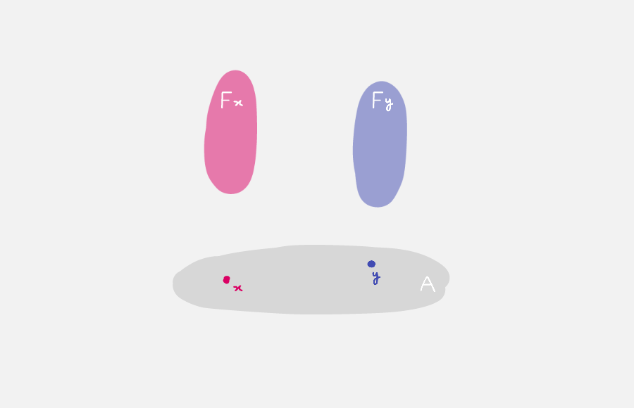
Introduce the dependent function version of rec_True called ind_True, similarly adding two rules to the system to describe it:
- ind_True : $\prod_{\mathrm{C}:\mathrm{True} → \mathrm{U}}$ ((C *) → $\prod_{x:\mathrm{True}}$C x)
- For any terms C, y, the assertion “ind_True C y * = y” holds
If we view C(x):U as a proposition about x, then “ind_True” says: given any proposition C(x) about x:True, if proposition C(*) holds, then for any x:True, C(x) holds.
Readers can verify that the following type assertion indeed proves our proposition:
ind_True (λx:True → x eq *) refl* : $\prod_{x:\mathrm{True}}$x eq *
If you find these dependent function expressions confusing, just roughly know they express the axiom “True type has unique value *”. Or you can try playing with type theory formal systems in Deductrium—hovering over each term shows its type, which should greatly help understanding. Type theory is unlocked relatively late in Deductrium. Readers without time can go directly to Deductrium’s creative mode to experience it: click the type layer, enter expressions in the theorem list, and the system will automatically calculate their types. You can also enter type assertions like A : B and definitional equality assertions like A === B, and the system will automatically determine if the input assertions are correct. You can also use the form xxx := XXX to abbreviate XXX as xxx, and after definition you can use it in theorems that follow (add with the plus button). 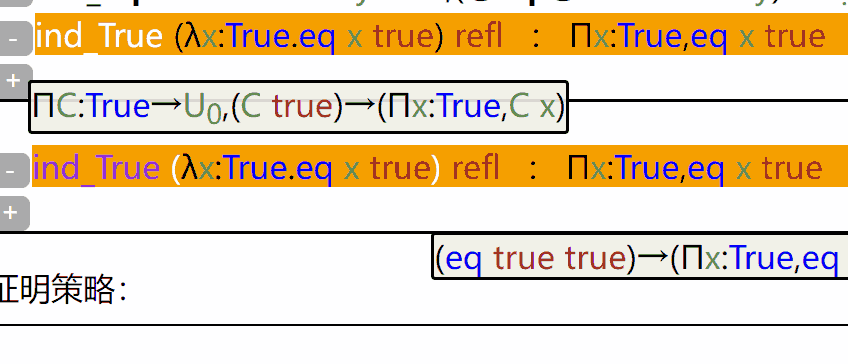
Now back to the main topic. Each type has corresponding induction principles, like “ind_Bool”, “ind_False”, even “ind_eq”, etc.
Let’s roughly describe what they represent without writing out their types and computational rules.
- ind_Bool: For any dependent type C(x), given values for C(0b) and C(1b), we can construct the dependent function $\prod_{x:\mathrm{Bool}}$C(x);
- ind_False: For any dependent type C(x), without giving any values, we can construct the dependent function $\prod_{x:\mathrm{False}}$C(x);
- ind_eq: Given type A, for any dependent type C(x:A,y:A,m: x eq y), given C(x,x,reflx), we can construct the dependent function $\prod_{x,y:\mathrm{A}}\prod_{m:\mathrm{x eq y}}$C(x,y,m);
Note 1: ind_False here actually implies the “principle of explosion”: for any proposition, we can construct a function that takes a False type variable and outputs it, so once we have a value of False type, we can prove everything.
Note 2: The eq type isn’t actually a simple type—it’s a complex type with three parameters A, x, y. However, it has only one construction method: refla : a eq a. So to construct functions about eq type, we only need to consider the case where x=y (definitionally equal).
Similarly, we can inductively define these complex types with parameters:
- Ordered pairs, also called product types: (a,b) : A × B, constructed by a constructor with two parameters (a:A and b:B). To construct type A × B we must give elements of both A and B, so A × B can be translated as the proposition “A and B”.
- Dependent product types: if a:A and b:B(a), then (a,b) : $\sum_{x:A}$ B(x). Its constructor type changes from simple functions to dependent functions. Since we only need to give any pair a:A and b:B(a) to construct the dependent product type, $\sum_{x:A}$ B(x) can be translated as “there exists x:A such that B(x) holds”.
- Sum type A + B, similar to boolean type, has two constructors: either constructed by the first constructor with parameter a:A, or by another constructor with parameter b:B. To construct type A + B we need either an element of A or an element of B, so A + B can be translated as the proposition “A or B”.
Since they’re all inductive types, they all have corresponding “ind_xxxx” functions without exception. They all assert that given a proposition C(x) with parameters, as long as we case-analyze all situations for all constructors of these inductive types, we can prove that for any x, proposition C(x) holds. I won’t expand on the specific details here.
Natural Numbers and Mathematical Induction
Finally, let’s look at the natural number type nat : U, which has two constructors “0” and “succ”:
- 0 : nat
- succ : nat → nat
What does this succ mean? It says if n is a natural number, then succ n is too. That is, parameters in inductive types can be recursive, and constructors of two inductive types can even “cross” construct, etc. Therefore, the number of constructors doesn’t equal the actual number of elements in that type. The ind_nat function is exactly equivalent to mathematical induction: to prove a proposition C(n) holds for all natural numbers n, we need to prove it holds for 0 (i.e., C(0)) and for succ. Since succ has parameters, we need to prove that for all x: nat, the proposition holds for succ x ($\prod_{x:nat}$ C(succ x)). However, the recursive nature of natural numbers isn’t reflected yet: all elements can only be generated from 0 or succ, so the x in succ x must already be a natural number satisfying the proposition, i.e., we actually have the given condition C(x) from recursion. Adding this gives $\prod_{x:nat}$C(x) → C(succ x). Now it’s identical to mathematical induction: first prove C(0) holds, then prove that for any natural number x, “from holding for x we can deduce it holds for x+1 (i.e., succ x)”.
The above uses a propositional perspective to understand the ind_nat function. Now let’s re-examine it from a function evaluation perspective: to define a function f about natural numbers, first define its value at 0, f(0), then for any x, its value at succ x, f(succ x), can depend not only on x but also on the previous value f(x). This allows us to define recursive functions. Actually, addition, multiplication, exponentiation, and all primitive recursive operations can be written using the ind_nat function. Those interested can refer to Wikipedia.
Differences Between Type Theory and Classical Logic
Let’s summarize and compare type theory with set theory:
| Item | Type Theory | Set Theory |
|---|---|---|
| Hypothetical reasoning | Ordinary functions | Logical implication symbol |
| Negation | Proposition implies False | Negation symbol |
| Universal | Dependent functions | First-order logic quantifier “for all” |
| Existential | Dependent product types | Combination of quantifier “for all” and negation |
| And | Product types | Combination of negation and logical implication |
| Or | Sum types | Combination of negation and logical implication |
We find that first-order logic treats universal and existential, and and or similarly, while type theory treats them very differently. First-order logic belongs to “classical logic”, which accepts the law of identity ($a=a$), law of excluded middle ($A\lor\lnot A$), and law of non-contradiction ($\lnot(A\land\lnot A)$). However, type theory doesn’t accept the law of excluded middle. The law of excluded middle says: a proposition is either true or false. This is obviously correct. Type theory is designed for computational mathematics, and every “evidence” in it is computable. Gödel’s incompleteness theorem says not all propositions are provable, meaning there exist propositions that can neither be proven nor disproven. When constructing “or” evidence in type theory, we must specify which side’s constructor to use for construction—this requires extra information. For Gödel propositions, obviously neither side can be constructed. Actually, many propositions without negation symbols are equivalent to the law of excluded middle and cannot be proven in type theory, such as double negation elimination:
- (¬¬A → A)
In contrast, type theory has no problem proving double negation introduction:
(λA:U. λx:A. λy:A → False. y x) : (A → ((A → False) → False)) = (A → ¬¬A)
Note that the law of excluded middle isn’t only implied by propositions with negation symbols. This seemingly harmless “Peirce’s law” also implies the law of excluded middle and thus cannot be proven: ((P → Q) → P) → P.
We could completely solve this problem by introducing axioms into type theory, but then computability would break down when encountering axioms. Actually, the law of excluded middle often isn’t needed to prove the vast majority of propositions. We’ll see later that homotopy type theory will disprove the law of excluded middle.
Determining Common Negation Problems
Have you wondered how to prove 0 ≠ 1 in type theory? We can only use indirect methods: first use “ind_nat” to define a function f : nat → U that maps 0 to True and 1 to False, then use the assumption that 0 equals 1 to get through ind_eq that if f(0) holds then f(1) holds, thus obtaining that proposition False holds. Actually, all constructors can use similar methods to attach different truth values to derive contradictions. This is called the universal property of inductive type constructors—“disjointness”.
Introduction to Homotopy Type Theory
Roughly speaking, homotopy type theory is the theory specifically studying equality types. It points out that types can be broadly classified into the following categories based on the properties of equality types:
- Types A that are like mere propositions: Similar to the True type, A has only one element, and for any a, b : A, we have a eq b holds.
- Types A that are like sets: For any a : A, the elements of type a eq a are unique.
- Other higher homotopy types: For any a : A, the elements of type a eq a include not only refla but possibly other things not equal to it.
Here’s the explanation:
- For propositions, regardless of what the evidence is, it only represents that it holds, without needing other extra information. Therefore, a “mere” proposition’s type should satisfy that all internal elements are equal.
- For sets, we no longer require only unique elements, but each element is like an isolated point without other extra structure.
- Higher homotopy types can be viewed as topological spaces: each value is a point in the space, definitionally equal values are viewed as the same point, propositionally equal but not definitionally equal points are viewed as having a path connecting them, and the evidence of propositional equality is these paths. Paths can also be judged for equality—equal paths are homotopic in the topological space—meaning there exists a higher-dimensional path linking them—a two-dimensional surface that allows one path to continuously deform into another path on it. If there exist paths different from refla, it means a loop starting from point a cannot continuously contract to a point.
Why can we view equality types as paths? It’s easy to construct proofs of reflexivity and transitivity of equations through the “ind_eq” function, i.e., construct functions:
- (x eq y) → (y eq x)
- (x eq y) → ((y eq z) → (x eq z))
These functions correspond to inverse and concatenation operations on homotopy paths. If readers aren’t clear about what homotopy is, they can refer to “Introduction to Algebraic Topology (Part 1): Homotopy Theory”.
The “Univalence” Axiom
But besides the unique evidence refl of equation reflexivity, what exactly are these other things? Homotopy type theory adds the “univalence axiom”—abbreviated as ua. First, we define that if two types can have bijective functions defined between them, these two types are called equivalent, denoted as “A ≃ B”. The specific definition expression involves some dependent ordered pairs (the dependent product types introduced earlier), containing bijective functions and evidence that they’re indeed bijective, etc. It’s somewhat complex to write out—please refer to the HoTT (Homotopy Type Theory) book. The ua axiom asserts the following proposition holds:
(A ≃ B) ≃ (A eq B)
Note the equivalence symbol represents bijection, which has two directions. One direction says there exists some value with type:
- idtoeqv : (A eq B) → (A ≃ B)
This is obvious—any type can define a bijection to itself. Here we stipulate choosing the simplest identity mapping, i.e., input a $refl_A$ (evidence of A eq A), and the idtoeqv function gives the identity mapping from A to itself, i.e., evidence of A ≃ A.
The other direction cannot be proven without adding axioms, so we need to add the following axioms to the system:
- ua : (A ≃ B) → (A eq B)
- ua and idtoeqv are inverse mappings of each other
This means each different bijection between types A and B corresponds to different evidence that types A and B are equal. In particular, the identity mapping corresponds to refl.
Besides introducing the “univalence” axiom, homotopy type theory also introduces inductive types for higher equality type constructors. Below we give the constructors for the circle $S^1$ as an inductive type:
- base : $S^1$
- loop : base eq base
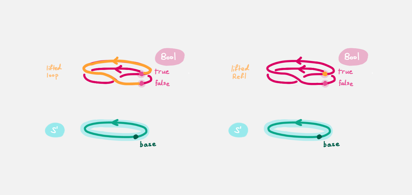
Note that loop here is different from refl (we’ll prove this shortly). We understand refl as a path on the circle contracted to a point, and loop as a path going clockwise around the circle once. The evidence for reflexivity and transitivity of equations corresponds to path inverse and path concatenation. Through them we can generate the entire fundamental group on the circle, i.e., all possible cases for values of type base eq base. Note that to define functions on type $S^1$ (i.e., ind_S1), besides specifying the function’s value at base, we must also specify where to map that loop.
With ind_$S^1$, we can prove that loop equals refl leads to contradiction, just like proving 0 ≠ 1. I’ll provide a possible approach: use ind_$S^1$ to define a function f : $S^1$ → U that maps base to the boolean type Bool : U. According to the univalence axiom from the previous section, we know the equality type Bool=Bool also has two elements: one is refl, the other is generated by the automorphism g that swaps 0b (false in the image below) and 1b (true in the image below), denoted as ua(g) : Bool=Bool. 
We now map loop to ua(g). Since we assume loop=refl, this function transfers the equivalence relation into Bool, obtaining that p : Bool=Bool generated by the automorphism swapping 0b and 1b equals refl : Bool=Bool. However, when we try to use these two equality relations to map variables in Bool type, the results are different. By assumption they should be the same, thus obtaining 0b=1b.
The constructors for the sphere $S^2$ : U as an inductive type are:
- base : $S^2$
- loop : reflbase eq reflbase
Homotopy type theory can even develop theories to calculate parts of the homotopy groups of hyperspheres $\mathbb{S}^n$. I really don’t have the energy to get that far, so I can’t introduce it here.
Homotopy Type Theory and the Law of Excluded Middle
After homotopy type theory adds the axiom “ua”, the law of excluded middle no longer holds. That is, we can construct a value of the following type:
“( $\prod_{A:\mathrm{U}}$ (A + (A → False)) ) → False”
We previously said the law of excluded middle is equivalent to double negation elimination, so we only need to give a specific f : $\prod_{A:\mathrm{U}}$ ((A → False) → False) → A, and obtaining a value of False type completes the proof of the original proposition (I’ll leave the conversion steps for readers to think about).
Let’s construct this specifically: examining elements of (Bool → False) → False, we know “Bool → False” is a false proposition. According to the principle of explosion (constructed by ind_False), we can obtain that any proposition holds. Therefore, given any x:Bool → False, we can deduce not only False but also that u(x) and v(x) are equal for any two elements u, v in (Bool → False) → False. In other words, functions u and v have the same output for any input x, so by the function extensionality axiom (obtainable from homotopy type theory axioms), we can prove u and v are equal, i.e., all elements of (Bool → False) → False are equal to each other.
With this foundation, we can now formally construct the contradiction. We said we need to construct a specific f : $\prod_{A:\mathrm{U}}$ ((A → False) → False) → A, and obtaining a value of False type (contradiction) completes the task. Let’s examine f(Bool), which has type ((Bool → False) → False) → Bool. For boolean type Bool, we construct function e : Bool → Bool through ind_Bool such that: e(0b)=1b, e(1b)=0b. (It’s this again constructing counterevidence!) It’s easy to see that function e is a bijection from Bool type to Bool type, i.e., we have (Bool ≃ Bool) holds. According to the ua axiom, ua(e) is evidence of (Bool eq Bool), and it’s different evidence from ua(id)=reflBool obtained from the identity mapping id.
Function f not only maps values of type A to ((A → False) → False) → A, it also maps equality paths on A to equality paths on the latter. We see that since type (Bool → False) → False has only one value, both refl and ua(e) in Bool will be mapped to the unit path refl of that value. For any u:(Bool → False) → False, according to the equality mapping transfer relation (see section 3.2 in “HoTT” for specific details), we have e(f(2)(u)) = f(2)(u), but function e is the mapping that swaps 0b and 1b, not the identity mapping, leading to contradiction.
Constructing Mere Propositions Through “Truncation”
We see that the root cause of the law of excluded middle not holding is that Bool type has extra elements while type (Bool → False) → False has only a single element. For those mere proposition types mentioned earlier, no contradiction would arise, so we can introduce a “narrow” law of excluded middle axiom in homotopy type theory:
LEM : $\prod_{A:\mathrm{U}}$ isProp(A) → (A + (A → False))
isProp(A) means “A is a mere proposition type”, i.e., any two elements in A are equal, abbreviated as $\Pi$x:A,$\Pi$y:A, x eq y. Note the condition “A is a mere proposition type” is necessary, otherwise as we analyzed earlier it would lead to contradiction.
The A+B corresponding to propositional logic A or B has two different constructors, so it’s not a mere proposition. Through higher-order inductive types with parameters, we can introduce a “truncation” mechanism to forcibly define a new type to make it a mere proposition:
For any A:U, we have:
- For any a:A, we have |a| : ||A||;
- For any x,y:||A||, we have x eq y.
This way, adding “||” can turn all propositions into mere propositions, and then we can happily use the law of excluded middle.
Using these “truncation” techniques, we can easily define concepts like quotient spaces in topology (constructing new spaces by viewing certain points or paths in the space as equivalent). Many operations in topology can be translated into the language of homotopy type theory. For example, fiber bundles in topology, which we haven’t mentioned, actually correspond to dependent function types. Finally, the axiom of choice also has a type theory version, but it also needs to be introduced separately as an axiom…
References
Homotopy type theory is somewhat like grand unification theory—both are recent theories still under development. The field of machine proof is more mature. There are too many related topics for this article to cover completely. Interested readers please explore on your own:
- Online proof assistant LEAN
- LEAN tutorial
- Online proof assistant jsCoq
- Coq tutorial
- The HoTT Game (Homotopy Type Theory Game)
- Homotopy Type Theory: Univalent Foundations of Mathematics (HoTT ebook)
Finally, let me recommend the creative mode in Deductrium, a game I created.