Introduction to Algebraic Topology (Part 1): Homotopy Theory
Note: This article does not require readers to have a professional background in topology. The term “algebraic” might give the impression of something abstract and difficult to understand, so this article aims to provide an intuitive understanding of homotopy and homology in algebraic topology. Specific formal definitions and technical details can be found in any algebraic topology textbook.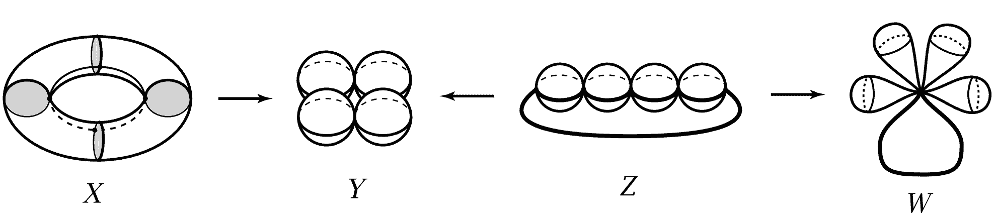
In “4D Space (X): Knots and Links“, we introduced various figures with holes in four-dimensional space. How to study and distinguish these holes is an important problem in topology. If you are not familiar with topological concepts like homeomorphism and isotopy, let’s briefly discuss these basic topological concepts first. Readers already familiar with these can skip ahead.
Introduction to Topology
Topology doesn’t concern itself with the specific dimensions and shapes of geometric figures; it only cares about how figures are connected. The first intuitive explanation is that as long as you can arbitrarily stretch a figure without tearing or gluing it, topologists consider the figures to be identical. Overly colloquial descriptions inevitably lose some details, so here’s a second-level explanation: two figures are topologically equivalent (technically: homeomorphic) if there’s a one-to-one mapping between every point in both figures, and the mapping is continuous.
It’s worth noting that while the first and second descriptions seem consistent, if we want to untie a knotted string with its ends glued together, we would have to cut the string, untie it, and then glue it back—but the second description doesn’t require the entire motion process between the two states to remain continuous, only that the two states can be continuously corresponded. So from the second perspective, a knot is equivalent to a circle, but not from the first perspective. Here we need to get used to a somewhat counterintuitive concept: when studying topological figures, we default to studying only the figure itself, not the external space it occupies. Thus when two figures are topologically equivalent, we call them “homeomorphic,” and when we talk about studying a “topological space,” we generally mean the figure itself, not the external space it occupies. But sometimes we do need to consider the space a figure occupies (for example, knots only exist in three-dimensional space and come undone in four dimensions or higher). In this case, we require that both the figures and their surrounding spaces undergo continuous mapping together. We say a trefoil knot and a circle are not “isotopic” in three-dimensional space but are “isotopic” in four-dimensional space. Compared to the first level, the second level of description can also handle things involving limits and infinity, which are difficult to “deform” intuitively. Let’s look at some examples:
- When mapping a circle to a broken circle, there’s a discontinuity at the opening, which topology doesn’t allow, so a circle and an arc are not homeomorphic.

The shapes of the letters O and Q are not homeomorphic, because if Q’s tail maps to a point on O, then that one point on O corresponds to all points on Q’s tail, violating the one-to-one correspondence. If Q’s tail maps to a small arc on O, then it overlaps with Q’s circle, also violating the one-to-one mapping requirement.
Any open interval $(a,b)$ is homeomorphic to the real line (understood as the real number axis $\mathbb{R}$), because the function $f(x)=\tan(x)$ maps points in the interval $(-\pi/2,\pi/2)$ one-to-one to $(-\infty,\infty)$, and the arctangent function value is also unique, satisfying the one-to-one correspondence condition. For any other open interval $(a,b)$, it can obviously be scaled and translated to the interval $(-\pi/2,\pi/2)$. Note that the closed interval $[a,b]$ is not homeomorphic to the real line, because the closed interval contains endpoints $a$ and $b$, which cannot find corresponding points on the real line.
The plane is homeomorphic to a sphere with one point removed. We can construct this homeomorphism through stereographic projection: except for the north pole, every point on the sphere can be uniquely projected onto the tangent plane at the south pole.
The idea that the plane is homeomorphic to a sphere with one point removed, or that any open interval is homeomorphic to the real line—these infinite figures being homeomorphic to finite figures—might feel abstract at first. But with more exposure, they too can become part of your intuition. In fact, many seemingly counterintuitive aspects of topology make sense upon reflection. In our learning process, intuition is constantly evolving.
Finally, let’s discuss the concepts of connected and path-connected. If a figure can be divided into a union of open sets with no intersection between them, it’s disconnected; otherwise, it’s connected. Intuitively, the entire figure is connected if it’s all in one piece, or equivalently, if any two points in the figure can be connected by a path within the figure. These two descriptions should seem equivalent, but intuition sometimes fails with infinity—there exist “pathological” figures that are connected but not path-connected. We won’t worry about them in this article; we’ll only consider more normal spaces. For example, a sphere is connected because any two points on the sphere can be connected by an arc; the set of integers is not connected because it consists of many isolated points. We call each connected part of a disconnected figure a connected component.
We will introduce homotopy and homology (due to length constraints, homology will be covered in the next article), both of which are tools for characterizing “holes” in topological spaces by constructing algebraic structures. Now let’s get to the main topic—homotopy.
Path Homotopy and the Fundamental Group
How do we define the concept of a “hole”? Let’s first look at the two-dimensional case. The figures below have one, two, and three holes respectively—simple, right?
However, the torus $T^2$ in three-dimensional space, shaped like a donut, is a closed surface without boundary. Intuitively it does have a hole—how do we describe this kind of hole? In “4D Space (X): Knots and Links“, we said the hole in a torus $T^2$ is one-dimensional because a one-dimensional line can pass through it, while the holes in the two-dimensional regions above are zero-dimensional because they can only contain a point. This previous approach isn’t actually very good for topological research: the hollow circle $S^1$ clearly has a hole—if placed in two-dimensional space, the hole can only contain zero-dimensional points; in three-dimensional space, a line can pass through; in four-dimensional space, a plane can pass through. Our research shouldn’t depend on the external space of the topological figure; it should depend on the topological space itself. Rather than using figures in external space to pass through these holes, it’s better to draw figures within the space to “wrap around” the holes. For example, the upper and lower rows in the figure below show homeomorphic figures. From the first row, we can see 0, 1, and 2-dimensional surfaces passing through holes from left to right, but through the second row, we clearly see that we can use 2, 1, and 0-dimensional figures to “wrap” the holes respectively: on the left, a sphere can wrap around a bubble; in the middle, a circle can be looped around the hole in the circle; on the right, two points can be restricted to two disconnected regions.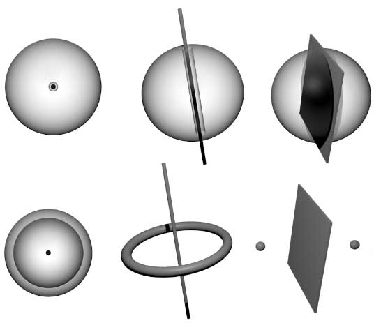
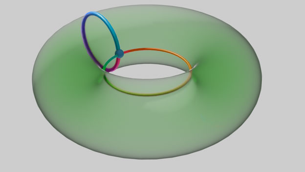
Another advantage of using figures inside the topological space that don’t depend on external space is that it makes the definition of holes clearer. Intuitively, the torus $T^2$ has only one hole, but actually it has two holes, corresponding to the blue and red meridian and parallel circles below.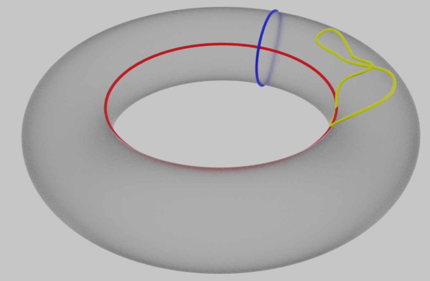
The red parallel circle directly loops around the hole in the middle of the torus. Since the torus is formed by rotating a hollow circle, the blue meridian circle actually loops around another hole. Intuitively, figures not caught by holes (like the yellow circle above) can be continuously deformed within the figure to shrink to a point, while figures caught by holes cannot be continuously contracted to a point. Again, I emphasize that all free movement here refers to movement within the space of the figure—here the figure is just the surface of the torus, so paths cannot be drawn outside the torus surface, i.e., cannot leave the torus surface to go into the interior or exterior three-dimensional space. If the figure we’re studying were a solid tire-shaped three-dimensional region, then circles could enter the interior, so the hole corresponding to the blue circle would be filled (the blue circle would thus become contractible to a point), leaving only the hole corresponding to the red circle.
Now although we can find some circles that loop around holes, many paths with different specific shapes and numbers of loops can be drawn on the same hole. To study this clearly, we naturally need to determine whether two circles describe the same hole in some sense, i.e., establish some equivalence relation between path circles. Let’s introduce the concept of path homotopy equivalence: if one path can be continuously deformed into another path within the figure, we consider them homotopy equivalent. Note that although these paths are generally circles, we only care about how the paths wrap around the surface, not about the self-intersections of the paths. So a more appropriate way to put it is that these closed path circles are continuous mappings from the standard circle to the figure we’re studying. Multiple points can map to the same point, so paths can self-intersect, meander, or even shrink to a point. The precise definition of homotopy equivalence is actually the equivalence relation that these mappings can vary continuously between. Paths that can shrink to a point are boring; those paths that cannot shrink to a point provide valuable topological information, like the meridian and parallel circles on the torus. We naturally wonder what all the homotopy equivalence classes of paths on the torus look like. Besides meridian and parallel circles, are there other non-contractible path circles? We can try to construct more complex paths starting from these two circles. For example, going around the parallel twice, or first going around the parallel once, then around the meridian once, composing to get a larger path.
Between these equivalent circles, as long as they pass through a common point, we seem to be able to define an “addition” operation: after completing one circle path and returning to the common point, we then follow another path, connecting them to form a larger circle. Note that paths are essentially mappings with direction. We might as well define the inverse operation of addition—subtraction: as long as we reverse the original path and walk backwards, we cancel out one circle. Those paths that can shrink to a point are equivalent to “0” in addition: adding any such path is the same as not adding it. We say paths that can shrink to a point are “null-homotopic“, denoted $a + 0 = a$. Note that null-homotopic paths within the same path-connected component of a figure are all homotopy equivalent.
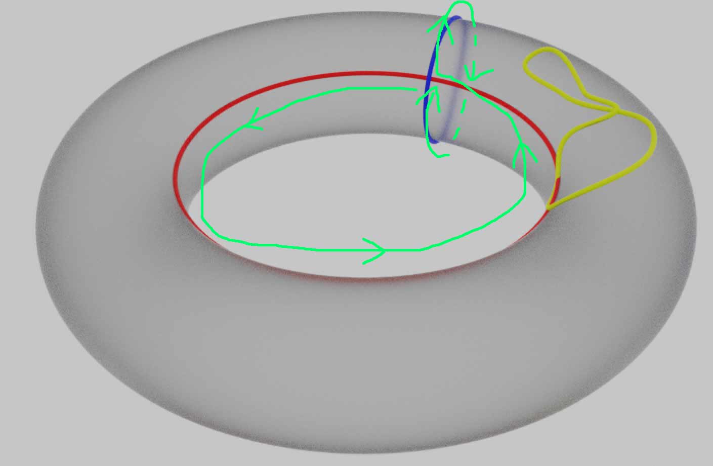
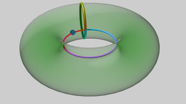
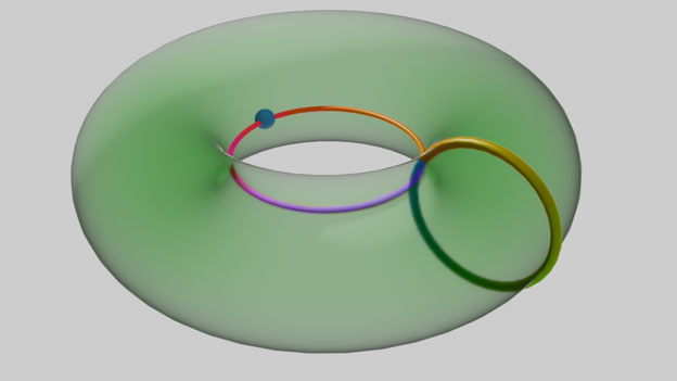
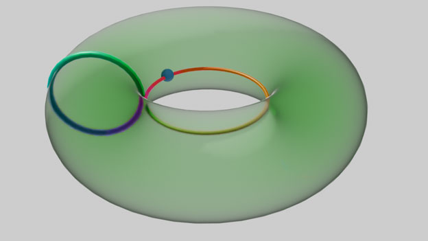
All homotopy equivalence classes of path circles starting from the same fixed point form an algebraic structure called the fundamental group (or homotopy fundamental group) through the addition operation. Note there’s an additional requirement here to start from the same fixed point (like point P in the figure above), which is stronger than general homotopy requirements. We call this “basepoint homotopy,” and all the addition operations we discuss later are for basepoint homotopy. It can be proven that all paths on the torus passing through a fixed point, in the sense of basepoint homotopy equivalence, can be obtained through addition and subtraction between meridians and parallels. This addition satisfies commutativity: we just need to show that $a+b$ and $b+a$ can be continuously deformed into each other. Here we show the mapping relationship with the circle through colors. We map the circle in the order red-orange-yellow-green-cyan-blue-purple, so the figure below represents meridian + parallel. By continuously moving the meridian around the parallel for one complete loop, the path finally becomes parallel + meridian.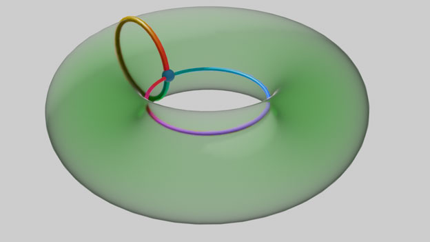
The addition between meridian and parallel circles on the torus satisfies commutativity, but for general homotopy paths this isn’t necessarily true. Generally speaking, the fundamental group is an algebraic structure that does not satisfy commutativity. For example, the figure below with two holes clearly has two non-homotopy equivalent circles passing through point P. It can be proven that the addition of these two circles doesn’t satisfy commutativity—the two paths below are not basepoint homotopy equivalent. Note that generally choosing different positions for the base point doesn’t affect the algebraic structure of the fundamental group, because the base point can drag paths and continuously change to another position within the same connected component, so we don’t need to worry about choosing the base point position.
Homotopy Between Topological Spaces
Actually, the first level explanation of topological equivalence says we can arbitrarily stretch figures without tearing or gluing. However, under this broad requirement, figures might only be homotopic rather than homeomorphic. For example, the letters Q and O are not homeomorphic because the intersection of Q’s tail with the circle is a three-way junction point, but no such point can be found on the letter O. But according to the principle of “no tearing or gluing,” we can definitely make Q’s little tail continuously shorter until it shrinks to a point on O—they are equivalent in some sense. However, homeomorphism doesn’t allow the letter O to grow a tail, because no points in O can be mapped one-to-one to points on the tail. Let’s introduce the concepts of deformation retract and homotopy equivalence: if a figure can be continuously deformed within itself to some subregion of the figure under the premise of “no tearing or gluing,” then this subregion is a deformation retract of the original figure. Figures before and after deformation retraction are homotopy equivalent and don’t change the fundamental group.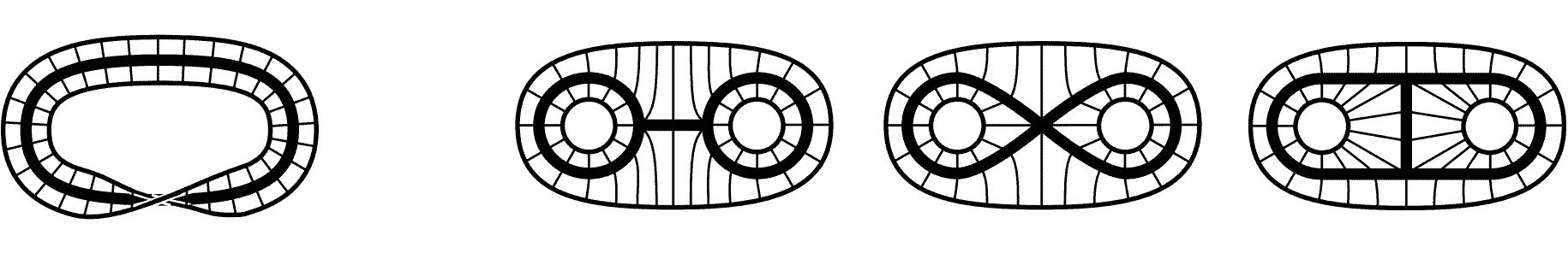
As another example, the figure of a torus $T^2$ plus four disks is homotopy equivalent to the figure of four spheres and a circle glued to a point.
Note that homeomorphism implies homotopy, but homotopy doesn’t necessarily imply homeomorphism. Here’s an interesting example from a topology textbook: if we view the shapes of Arabic numerals 0-9 as one-dimensional figures in the plane, then by homeomorphism the numbers can be divided into 5 classes: {0}{12357}{4}{69}{8}, but by homotopy there are only 3 classes: {12357}{0469}{8}.
Figures that are homotopic to a point are called “contractible”—they’re the simplest figures in the homotopy sense. For example, all solid polyhedra and spheres without holes have a point as their deformation retract. The figure below that looks like two layers of cardboard boxes or rooms is also contractible. Can you imagine the process of it shrinking to a point?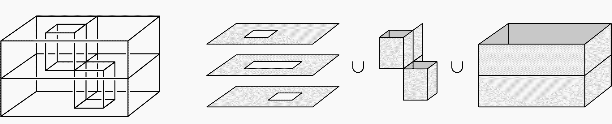
Actually, these two layers of “rooms” can be obtained by continuous deformation from a solid rectangular block: imagine digging a vertical shaft from the top surface of a solid cube, digging straight down to the lower half to hollow out the entire lower level, then similarly, digging a hole from the bottom surface of the solid cube, digging straight up to the upper half to hollow out the entire upper level. The two excavations don’t break through to each other; they’re separated by some surfaces, giving us exactly this figure. A solid cube (which is homeomorphic to a solid ball $D^3$) is contractible, so this figure is also contractible. It seems that complex figures can’t be understood by eyes alone.
Van Kampen’s Theorem and Computation of Fundamental Groups
We mentioned earlier that addition between meridian and parallel circles on the torus has commutativity, while addition between paths around two holes in a two-dimensional region doesn’t have commutativity. Let’s use the language of group theory to describe the structure of these two fundamental groups. The basic concept of group theory is simple: it’s a set with an operation that satisfies closure, associativity, has an identity element and inverses. See “Group Theory Series (Part 1): Introduction to Group Theory“ for details. Note that we previously used addition to represent path composition; now we’ll switch to multiplication: $a^n$ represents the composition of $n$ paths $a$, $a^{-1}$ represents the reverse path $-a$, and contractible circles (the additive identity 0) are now written as 1 (multiplicative identity)—just a change of notation that doesn’t affect the mathematical essence.
The torus and the two-dimensional region with two holes both have two basic paths a and b as generators of the fundamental group, meaning all other paths can be obtained by their composition. For the torus, the generators satisfy the commutative condition $ab=ba$, and all paths in the torus can be written as $a^mb^n(m,n\in \mathbb{Z})$ (reminder: $\mathbb{Z}$ is the set of integers), where m and n are obviously the number of loops around the meridian and parallel respectively. The fundamental group of the torus is commutative, and its Cayley graph (which shows how to get the entire group from generators) is a two-dimensional grid, where the horizontal and vertical coordinates are the respective loop counts around meridian and parallel. This group is denoted $\mathbb{Z}\times \mathbb{Z}$. Remember the direct product figures that satisfy commutativity (discussed here)? Actually, two groups $A$ and $B$ can also undergo direct product operations: using lowercase letters $a$ and $b$ to denote elements in groups $A$ and $B$ respectively, each element in the direct product group is an ordered pair $(a,b)$, with multiplication rule: $(a_1,b_1)(a_2,b_2)=(a_1a_2,b_1b_2)$. In fact, the fundamental group of a direct product shape is exactly the direct product of fundamental groups! The fundamental group of a circle is the integer addition group, so the fundamental group of the torus is the direct product of two integer addition groups.
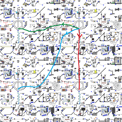
For the two-dimensional region with two holes shown below, there are no cancellation conditions between the two path generators—that is, besides the basic rule that walking backwards cancels a loop (i.e., $a^{-1}a=b^{-1}b=aa^{-1}=bb^{-1}=1$), path compositions with different orders are all non-homotopic circles. Therefore, all possible path combinations result in different group elements. This is a group that can be generated from two paths to contain the maximum number of elements—mathematicians simply call it the free group, denoted $\mathbb{Z}*\mathbb{Z}$. The Cayley graph of this free group turns out to be a fractal.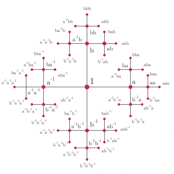
The only difference between the fundamental groups of the torus and the two-dimensional region with two holes is the constraint condition $ab=ba$. Since there’s only this small difference, there should be some connection between them. As shown below, a torus with one point removed is homotopic to two circles joined at a point (i.e., figure “8” shape), which is exactly the deformation retract of the two-dimensional region with two holes. We’ll soon see that removing a hole has an important impact on whether commutativity holds.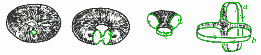
After removing a hole from the torus, the previously contractible green path in the figure becomes non-contractible. In the homotopy equivalent figure of two circles joined at a point (denoted as $a$ and $b$), the green path is $aba^{-1}b^{-1}$. Let’s look at it from another angle: the two circles joined at a point is exactly the deformation retract of the two-dimensional region with two holes removed. Its fundamental group, which we’ve already discussed, is freely generated by two paths a and b. But once we fill the hole (i.e., glue on a disk that covers the hole), the green path becomes contractible on the entire figure, i.e., $aba^{-1}b^{-1}=1$. Rearranging gives us $ab=ba$. “Filling” the hole reduces the number of non-contractible paths, which we denote as $\langle a,b|ab=ba\rangle$. Compared to the free group, it has the commutative constraint and is no longer “free.” If readers understand the first isomorphism theorem for groups, they’ll know that the group $\mathbb{Z}\times\mathbb{Z}$ is exactly the quotient group of the free group $\mathbb{Z}*\mathbb{Z}$ obtained by mapping $aba^{-1}b^{-1}$ to 1. In fact, almost all common discrete groups have generator representations—they’re all isomorphic to subgroups of some free group.
This example of dividing the torus into a hole-filling disk and the remainder homotopic to two circles joined at a point inspires us that computing the fundamental group of complex figures might be possible by dividing the figure into parts, computing each part, then combining to get the fundamental group of the entire figure. Van Kampen’s theorem states that if a figure can be expressed as the union of two subfigures, and their intersection is path-connected, then we can obtain the fundamental group of the entire figure from the fundamental groups of the two subfigures through a “free product” and then quotient out some constraints (i.e., construct a quotient group). The free product of groups $A$ and $B$ is denoted $A*B$. What is it? Similar to free groups, it means constructing a larger group from two groups where elements from different groups don’t satisfy commutativity and there’s no way to simplify. But since the two figures share common parts, the non-contractible paths on these can serve as “bridges” to simplify some originally non-contractible circles on both sides. For example, the intersection of the punctured torus and the hole-filling circular patch has that green circle as its deformation retract. Since the green circle is contractible on the circular patch, it becomes contractible on the entire figure. Let’s practice by computing the fundamental groups of the complement spaces of a circle, two disjoint circles, two linked circles, and a torus knot in three-dimensional space $\mathbb{R}^3$. Note: complement space means the part remaining after removing the original figure from the entire space (here three-dimensional space $\mathbb{R}^3$).
First, let’s look at the deformation retract of the complement of a circle. It’s equivalent to a sphere with a line through it, which can be further deformed to get a figure with a sphere and circle joined at a point (this way of constructing new figures by gluing at a point is called a wedge sum). We divide this figure into sphere and circle parts. All paths on the sphere are contractible, and paths on the circle can wind n times. Their common part is a point. The sphere doesn’t add any new non-contractible circles, so the entire figure has the same fundamental group as the circle, both isomorphic to the integer addition group $\mathbb{Z}$.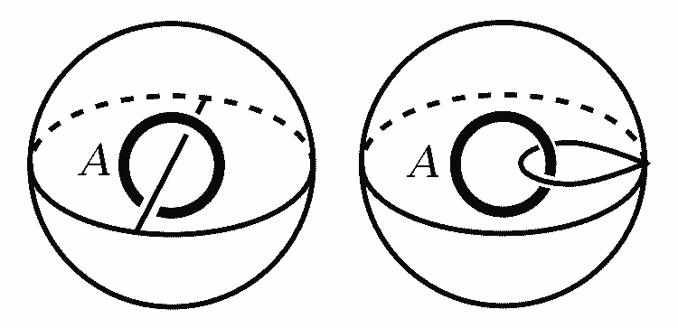
The complement of two disjoint circles can actually be seen as the union of two complements of single circles above. They intersect in a plane in the middle, and planes are also contractible to a point, so the entire space is the wedge sum of two spheres and two circles. Paths on spheres are not non-contractible, so there are only paths winding around the two circles. There are no other cancellation conditions between them, yielding the two-generator free group $\mathbb{Z}*\mathbb{Z}$.
For linked circles, they can be separated by a torus—this might be hard to imagine, but if we put it in the stereographic projection of the Hopf fibration on the 3-sphere, things become clear: two linked circles correspond exactly to the north and south poles on the 2-sphere, and any latitude circle separating them corresponds to tori on the 3-sphere. These tori appeared in episode 8 of “Dimensions: A Mathematical Walk.” Since it’s a torus, its fundamental group is $\mathbb{Z}^2=\mathbb{Z}\times\mathbb{Z}$.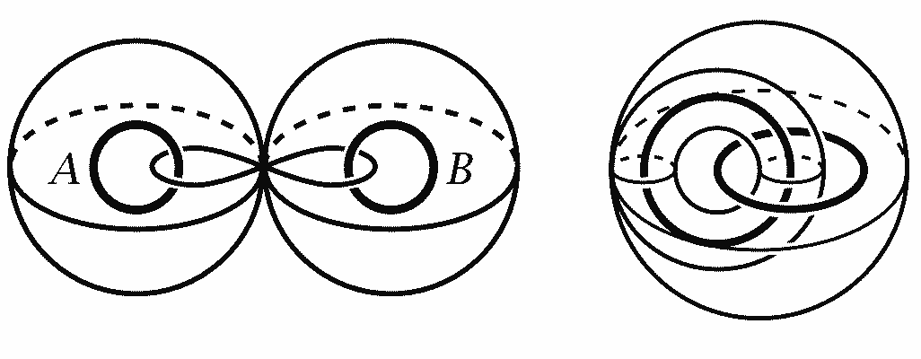
We see that the fundamental group of the complement of disjoint circles is larger than that of linked circles—linking the circles makes some non-contractible paths become contractible. Matrix67’s blog post mentions an interesting mathematical magic trick that exactly reflects the difference between these two homotopy groups:
Thus, a small magic trick is born. As shown in the left figure below, wrap a thin wire loop around two safety pins—you can easily verify that this wire loop cannot be removed. Now, pin the two safety pins together, and the wire loop miraculously falls off by itself. (Can you see why?)

Note that in these three examples, the common parts of the two parts of the deformation retract are all just a point, containing no other non-contractible paths, with no “bridges” to simplify paths on both sides. So the entire figure is directly the free product of the two groups. A sphere is a simply connected figure where all paths are contractible, with fundamental group containing only the identity element 1. The free product of 1 with any group is still 1.
Finally, let’s tackle something complex: computing the fundamental group of the complement of a torus p,q-knot in three-dimensional space. What is a torus knot? Due to the existence of meridian and parallel circles, we can describe points on the torus through meridian-parallel coordinates like on a sphere. If a moving point’s rate of change in meridian and parallel coordinates maintains a constant ratio, trajectories form on the torus. As long as the ratio is rational, it eventually forms a closed one-dimensional trajectory, which is usually knotted. The knot obtained from the rational number p/q is called a torus knot. For example, the left figure below is the simplest 2,3-knot (trefoil knot). Our torus doesn’t have to be in three-dimensional space—viewing three-dimensional space as the space obtained by stereographic projection from a hypersphere with one point removed, we can throw both the torus and knot onto the hypersphere surface. These figures have important significance in four-dimensional geometry, see cfy’s article for details. Actually, lifting to the hypersphere has advantages. For example, it’s hard to see directly that torus p,q-knots and q,p-knots are equivalent, but if we know that stereographic projection on the hypersphere can swap meridian and parallel lines on the torus, then this conclusion becomes obvious. According to hole dimension matching, holes formed by removing zero-dimensional points from three-dimensional regions must be wrapped by two-dimensional surfaces—one-dimensional paths don’t match and are all contractible (the deformation retract of a three-dimensional region with a zero-dimensional point removed is a sphere, where all paths are contractible). Therefore, we can safely add the point at infinity to study the fundamental group of the space on the hypersphere $S^3$ with the torus knot removed. We’ll see that placing it on the hypersphere simplifies the fundamental group calculation.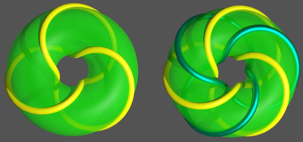
The torus naturally divides the hypersphere into two parts: one is the interior region of the torus, the other is the exterior region of the torus plus the point at infinity (because it contains the stereographic projection pole). They’re both solid three-dimensional tori, and the intersection of the two tori is the torus surface. In the complement space with the knot removed, the topological shapes of the two tori are unaffected, but their common part becomes the torus with the knot removed. As shown in the right figure above, the deformation retract of this common part is the same as the knot itself, both homeomorphic to a circle.
Now with two torus regions and their intersection—a torus with some regions removed that’s homotopic to the knot—we can use Van Kampen’s theorem: Note that the deformation retracts of the two solid three-dimensional tori are also circles, corresponding to the blue circle and red line in the figure below. Note the red line is also a circle, just stereographically projected through the pole. The fundamental group of a circle is the integer addition group $\mathbb{Z}$, so the fundamental group of the entire complement space is the free group generated by paths around the red and blue circles, quotiented by some simplifiable paths obtained using the common part as a bridge. Let’s see which paths between the two regions can be simplified.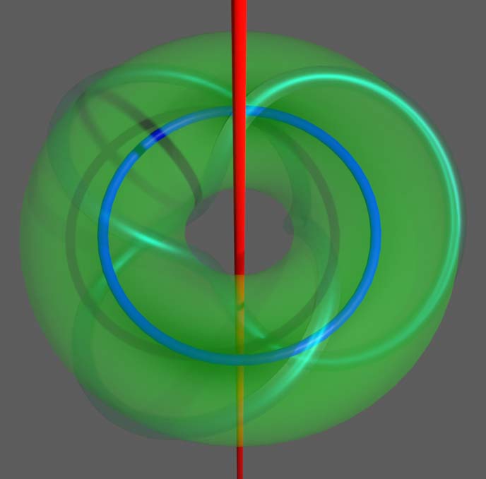
The common part of the two tori is homotopic to the trefoil knot. Observing carefully, it’s not hard to find that this trefoil knot path winds 2 times around one torus and 3 times around the other. Denoting the path generators around the red and blue circles as $a$ and $b$, the common region serves as a “bridge,” giving us $a^3=b^2$. This group is denoted $\langle a,b|a^3=b^2\rangle$. Similarly, we can obtain the fundamental group of a p,q-knot as $\langle a,b|a^p=b^q\rangle$. The Cayley graphs of these groups are somewhat difficult to draw, but I Googled and found someone has actually drawn them.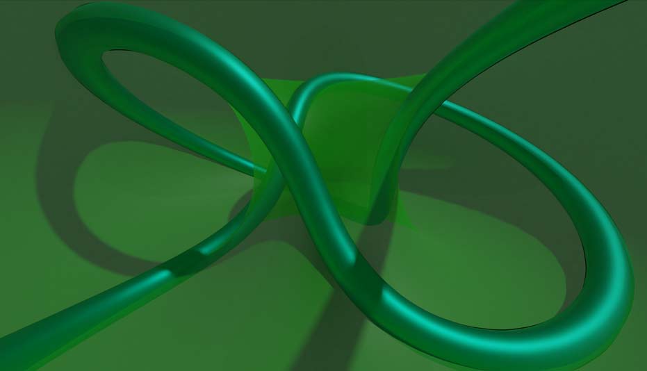
Covering Spaces and Path Lifting
We’ve been dealing with abstract fundamental groups all along. We’ll see that covering spaces, defined purely geometrically, have an intricate connection with fundamental groups—fundamental groups actually have strong geometric meaning. Imagine you’re in a circular corridor, and after going around once, you find you haven’t returned to the starting point but have arrived at a new place. You’d definitely feel very strange, as if you’d passed through a portal to a new world. Or imagine walking up a stairway only to find that going up brings you back to the lower floor where you started—this would also be quite frightening… You can check out this video on Bilibili which shows a double covering space formed by the complement of a portal frame removed from three-dimensional space. I’ll complain here that the video author doesn’t understand mathematics—the title says “non-Euclidean space,” but actually it has nothing to do with non-Euclidean geometry; it should be called a covering space. It seems the public thinks any space not homeomorphic to $\mathbb{R}^n$ is non-Euclidean…
Let’s look at the definition of covering spaces: A covering space consists of two spaces and a mapping between them: there exists a continuous mapping between the covering space $\tilde{X}$ and the base space $X$, such that the preimage of any point’s neighborhood in the base space $X$ consists of many disconnected parts in the covering space $\tilde{X}$, and each connected component is homeomorphic to that point’s neighborhood. Translating to understandable language: every point in the base space is covered by n layers in the covering space, and each layer locally looks the same as the base space. Here are some examples:
- An infinite helix projected along its axis gives a circle—this is an infinite-sheeted covering space of the circle.
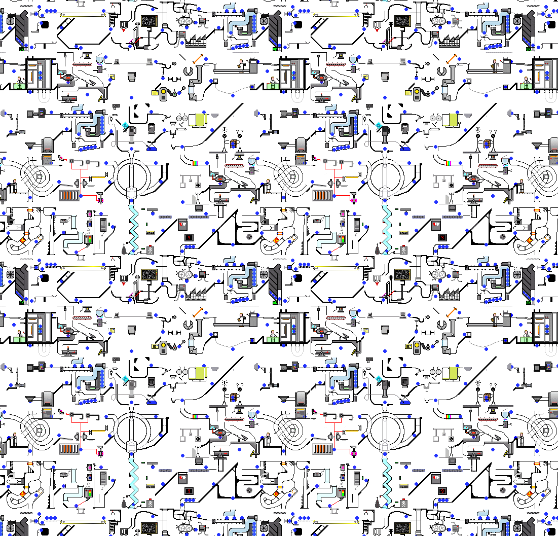
- Observe the balls in this amazing gif animation below—they exit the game boundary and appear from the opposite side. This topological structure is homeomorphic to a torus. Since top-bottom and left-right are connected, we can tile copies of the image across the entire plane. Everything in the image has infinitely many copies in this plane. According to the definition of covering spaces, the two-dimensional plane $\mathbb{R}^2$ is an infinite covering of the torus $T^2$. Actually, this animation only has 30 frames looping. Including the time dimension, the topology of the entire spacetime is a three-dimensional torus $T^3$, which is the direct product of three circles (homeomorphic to various toroidal cells), with fundamental group $\mathbb{Z}\times\mathbb{Z}\times\mathbb{Z}$.
A certain loop on the torus corresponds to infinitely many loops in the covering space. But if we fix the starting point of the loop in the covering space, then the path in the covering space is uniquely determined—this is the uniqueness theorem for path lifting in covering spaces. The endpoint and starting point of a loop in the base space are the same point, but in the covering space, the loop might be a path connecting two different points. It’s not hard to see that as long as we start from one point in the covering space and go to another point corresponding to the same point in the base space, after covering projection to the base space, we get mutually inequivalent non-contractible paths. Actually, covering spaces satisfying certain conditions can have a one-to-one correspondence with fundamental groups.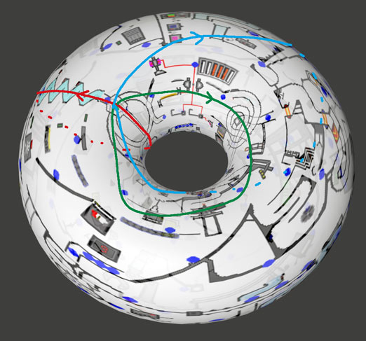
Classification of Covering Spaces and Universal Covering Spaces
What do the covering spaces of the wedge sum of two circles look like? We’ll give many, many covering spaces. These examples come from Allen Hatcher’s algebraic topology textbook.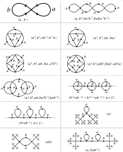
With so many covering spaces, is there one with the maximum number of sheets? Imagine if walking along any non-contractible circle would “transport” you to a new world—such a space would be the largest. We call it the Universal Covering Space, and it can cover all other covering spaces. Since all non-contractible paths in the universal covering space are lifted to become non-closed paths, there are no non-contractible paths left, so the universal covering space is simply connected with fundamental group 1. The shape of a figure’s universal covering space is very much like the shape of its fundamental group’s Cayley graph. For example, the universal covering space of the torus is the plane $\mathbb{R}^2$ we saw earlier, and the universal covering space of the wedge sum of two circles is a fractal with no loops at all, just like the Cayley graph of the two-generator free group we drew earlier.
We can see that as covering spaces get larger, fundamental groups get smaller. Actually, all covering spaces of a space correspond one-to-one with subgroups of the fundamental group, and normal subgroups of the fundamental group correspond to covering spaces with better symmetry… We won’t expand on this further here.
Introduction to Higher Homotopy Groups
Readers who have seen “4D Space (X): Knots and Links“ know that in higher-dimensional spaces, one-dimensional paths can’t necessarily loop around all holes because holes have different dimensions and must match to be caught. For example, we can’t use the one-dimensional fundamental group to capture the topological change before and after removing a point from three-dimensional space. Therefore, besides the fundamental group obtained from paths (circles), there are higher homotopy groups obtained from spheres and hyperspheres as higher-dimensional “paths.” These higher homotopy groups are sometimes particularly complex. Let’s look at the various homotopy groups of the circle:
First, the first homotopy group is the fundamental group of paths. For homotopy equivalence classes, there’s only the degree of freedom of the winding number around the hole. A path winding m times around the hole composed with a path winding n times gives a path winding m+n times. Therefore, the “addition” operation between these path equivalence classes is the same as integer operations, which we denote as $\pi_1(S^1)=\mathbb{Z}$. Here we use $\pi_i$ to represent the i-dimensional homotopy group, $S^1$ represents the one-dimensional sphere (i.e., circle), and $\mathbb{Z}$ is the symbol for the set of integers.

What is the second homotopy group of the circle? Can we map a two-dimensional sphere to a one-dimensional circle? Perhaps we could stretch the sphere into noodles to place on the circle, but it’s contractible—it’s null-homotopic. It can be proven that a two-dimensional sphere can’t loop around the hole in a circle, meaning there’s only one homotopy equivalence class: the null-homotopic mapping. We denote this as $\pi_2(S^1)=0$. Through covering space theory, we can deduce that higher-dimensional hyperspheres also can’t wrap around circles, so all higher homotopy groups of the circle are trivial groups containing only the identity element.

Now let’s study the various homotopy groups of the two-dimensional sphere: First, as a simply connected figure without holes, all one-dimensional paths on the sphere are contractible, so the first homotopy group is 0. The second homotopy group involves using the sphere to cover itself. Recall that a one-dimensional circle can cover itself n times. It can be proven (Hopf degree theorem) that the ways an n-dimensional sphere can cover itself can also be described by a winding number, and the homotopy group structure also corresponds to integer addition, denoted $\pi_n(S^n)=\mathbb{Z}$.
Note here how we define addition between higher-dimensional spherical “paths”: pinch the equator of a sphere to a point, and we get the wedge sum of two spheres. The reverse of this process is adding two spherical paths to get a new sphere. Because there are more dimensions, addition operations in dimension two and above can exchange positions in space, satisfying commutativity. But this doesn’t make higher homotopy groups simple. It seems we could similarly think that the third homotopy group of the two-dimensional sphere is also null-homotopic, but exceptions begin to appear. We want to construct a non-contractible mapping from the three-dimensional sphere to the two-dimensional sphere. Remember the Hopf fibration? In the Hopf fibration, each fiber on the three-dimensional sphere is a circle, corresponding to a point on the two-dimensional sphere. This is exactly a non-trivial way to map points on the three-dimensional sphere to the two-dimensional sphere. It can be proven that this Hopf map is non-contractible, and it can compose with itself. We can also count some kind of “winding number,” so the third homotopy group of the sphere $S^2$ is also the integer addition group $\pi_3(S^2)=\mathbb{Z}$. Are these “exceptions” common? Actually, the complex structure of higher homotopy groups is not exceptional—looking at the table below shows how terrifying higher homotopy groups are. Computing all homotopy groups of n-dimensional spheres is actually a very difficult problem in topology that remains challenging today.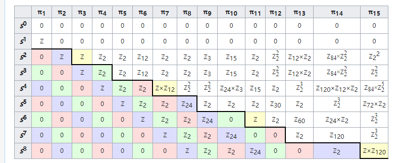
Solving homotopy groups is very difficult. Is there a simpler approach? In the next article, we’ll introduce a concept closely related to homotopy—homology. Unlike homotopy groups, it defines an addition operation that always satisfies commutativity, and computation is also relatively more convenient. (To be continued)