Introduction to Algebraic Topology (Part 2): Homology Theory
/// Note: This article only provides an intuitive understanding of homology-related concepts, without rigorous derivations. Corrections for any errors are welcome.
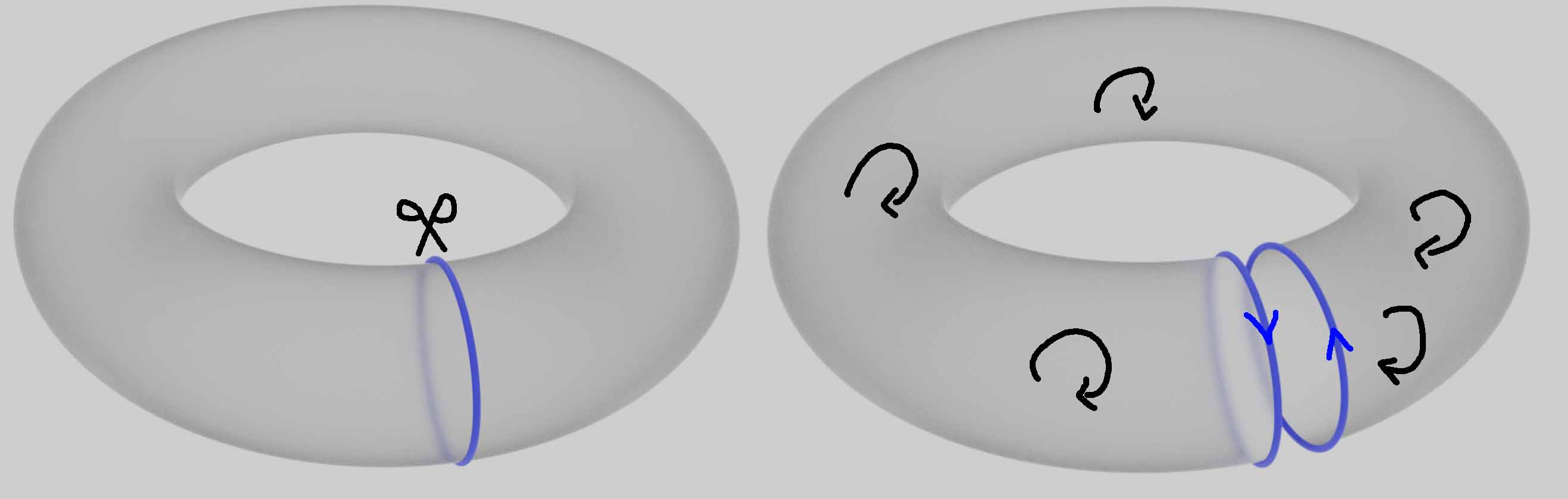
The previous article discussed Homotopy Groups. This time we’ll look at Homology Groups. Homology is somewhat more abstract, but in some ways simpler than homotopy. Returning to the initial idea of determining holes through paths, homotopy studies the process of continuous contraction of circles, which is direct but difficult to compute. Upon careful observation, we find that those shapes that can be contracted to a point all have closed regions inside. If we assume that whenever a closed path is the boundary of some region in the shape, then it hasn’t looped around or crossed any holes, we call such loops “nullhomologous.” Note that nullhomologous paths here are similar to contractible paths in homotopy, but nullhomologous paths may not actually be contractible - we’ll see that homology conditions are weaker than homotopy. For example, in the left figure below, the boundary of the cyan region contains the hole’s boundary and the red loop. The red loop alone is not the boundary of any shape, so we know it encloses a hole. In the right figure, the red loop is the boundary of the blue region, so it doesn’t contain any holes and is “nullhomologous.”

Following homotopy groups, we’ve roughly understood homology equivalent paths. To obtain homology groups, we need to define composition operations between them. First, let’s think about how homology equivalent paths should be specifically defined. Note that paths have direction, and the most important thing here is to carefully handle the relationship between closed regions and directions on boundaries. We’ll define the concept of “chains,” which are n-dimensional generalizations of directed paths.
Chains and Chain Groups
Informally speaking, an n-dimensional chain is defined as a mapping from any n-dimensional subshape in space to integers. This integer can be understood as the number of times shapes are stacked, and n-dimensional subshapes have direction - reversing direction also reverses the stacking count. Intuitively, n-dimensional chains describe directed, stackable n-dimensional subshapes. Since we’re already stacking, addition between chains naturally means adding their stacking multiplicities. Note that multiplicities can be positive or negative - same directions accumulate, opposite directions cancel. The figures below show addition between 1-dimensional chains and between 2-dimensional chains respectively. Note that chains of different dimensions cannot be added. These n-dimensional chains and their addition form an algebraic structure called the n-dimensional chain group. Note that addition between chains is essentially integer addition of stacking numbers, which of course satisfies commutativity, so chain groups and the homology groups we’ll define later are all abelian groups.
After defining chains and addition (chain groups), how do we describe holes? We need to determine somehow whether this n-dimensional chain is the boundary of some (n+1)-dimensional chain - if not, we’ve found a hole. Note that the boundary of any shape must be closed, i.e., the boundary of any shape has no boundary. Like studying homotopy groups, we only study closed chains, because non-closed chains naturally cannot be boundaries of higher-dimensional shapes. Note that chains have direction and stacking multiplicity, so chain boundaries also preserve direction and stacking multiplicity, i.e., taking the boundary of an (n+1)-dimensional chain yields an n-dimensional chain (we won’t consider non-smooth fractal extreme cases in this article). Readers might feel dizzy here, so let’s look at examples in various dimensions.
Zero dimension is a point, which might be the boundary (endpoint) of a 1-dimensional shape. According to the definition of homology, for two zero-dimensional points to be homologous, their difference must be the boundary (endpoints) of some 1-dimensional chain - in other words, they just need a path connecting them. Note that chains have direction, and points (zero-dimensional chains) and line segments (one-dimensional chains) also have directionality. Zero-dimensional chains are like scalars, representing point multiplicities (i.e., several points stacked together). One-dimensional chains are somewhat like vectors: segment $ab$ and segment $ba$ are opposite, and they cancel when added. We can write $ab = -ba$.
We introduce a boundary operator notation $\partial$ representing taking a chain’s boundary. We stipulate that the starting point is positive and the ending point is negative, i.e., $\partial(ab) = a - b$. Why give the endpoint a negative sign? Because we want the boundary operation and chain addition to be commutative: triangle $abc$’s boundary is a closed 1-dimensional shape with no boundary, consisting of three chains $ab + bc + ca$. Finding its boundary, we have $(a-b) + (b-c) + (c-a) = 0$, which matches expectations. Another reason for this convention: we said earlier that we want the difference between two points to be the boundary of some chain, so $a-b$ is naturally the boundary of the 1-dimensional chain $ab$, therefore the zero-dimensional chain $a-b$ is a zero chain, which can be written as $a-b = 0$ in the homological sense, thus $a = b$ (points $a$ and $b$ are homologically equivalent).
Now let’s do some exercises calculating boundary chains to see what 2-dimensional chains are.
- Calculate the boundary chain of the shaded 2-dimensional chain in the figure below. The chain’s direction is already marked.

We still record chain directions in triangular order. So the boundary chain to find is:
$$\partial(ade+aeb) = \partial(ade) + \partial(aeb) = (ad + de + ea) + (ae + eb + ba)$$
Note that $ea = -ae$, so we have $\partial(ade+aeb) = ad + de + eb + ba$, with the boundary shown below.
The boundary of any shape is closed - in other words, the boundary of a boundary must be 0, i.e., for any chain $A$ we have $\partial\partial A = 0$. Readers can verify that the red chain above indeed has boundary 0. - What is the boundary chain of the following 2-dimensional chain? Readers can calculate it themselves; the answer will be given in the next section.

Cycle Groups and Boundary Groups
Now that we’re familiar with arbitrary chains, addition between chains, and the boundary operation, the next step is to narrow our focus to closed chains that might loop around holes, i.e., chains satisfying $\partial A = 0$. We call these chains without boundaries cycles. We stipulate that zero-dimensional points have no boundary, so zero-dimensional chains are all cycles. We also said earlier that if a chain is the boundary of some shape, we still consider it as not looping around holes, i.e., for chain $A$ there exists chain $B$ such that $\partial B = A$. We call such chains $A$ that are boundaries of some chain $B$ boundaries. Why is this section titled “Cycle Groups and Boundary Groups”? Because we can verify that cycle + cycle = cycle, boundary + boundary = boundary - both types of chains are closed under addition, so they’re both groups. Also, since every shape’s boundary is a closed shape, all boundaries are cycles, so we have the group inclusion relation: Boundary Group $\subset$ Cycle Group $\subset$ Chain Group.
The figure below gives some examples: on the left, the cyan loop and black loop are both cycles and boundaries (cyan is the boundary of $acd+dea$, black is the boundary of $feb$), while the purple loop is a cycle but not a boundary (it loops around hole $fed$); the right figure has two 1-dimensional chains (blue and red) and one green 2-dimensional chain, none of which are cycles. Note that although the blue chain’s shape is closed, its directions are inconsistent - its boundary is $2e-2a$.
Homology Classes and Homology Groups
With the above foundation, homology classes can naturally be defined. We consider two cycles that differ by a boundary as the same, forming an equivalence class called a homology class. We can verify that addition between these equivalence classes is also well-defined. The addition operation between homology classes forms the homology group. If readers are familiar with the first isomorphism theorem for groups, it’s not hard to see that the homology group is the quotient group obtained by mapping boundaries in the cycle group to 0.
The concepts aren’t many, but the explanation is somewhat abstract. Let’s look at more examples to gradually understand.
As mentioned before, all points with the same multiplicity in the same connected component are homologous. To classify all zero-dimensional chains by homology equivalence classes, we just need to count the total number (multiplicity) of points in each connected component. For example, in a shape with three connected components where all points in each component are equivalent, we can combine like terms. All zero-dimensional chains can definitely be written in the form $ax+by+cz$. These zero-dimensional homology chains together with addition form the zero-dimensional homology group. Addition between them is just adding the coefficients in front of $x,y,z$, just like addition between integer ($\mathbb{Z}$) coordinate points in 3D space, which we denote as $\mathbb{Z}^3$. We can easily extend this to any topological space with $i$ connected components - its zero-dimensional homology group is $\mathbb{Z}^i$, i.e., isomorphic to the additive group of integer coordinates in $i$-dimensional space.

Here’s a reminder about the relationship between chain groups and homology groups: chain groups are simply all chains with addition operations, including all shapes whether closed or not, and chains change when the shape changes; while homology groups are addition operations between homology equivalence classes constructed within cycle groups, reflecting the topological information of the shape. Imagine if we directly defined addition on zero-dimensional chain groups - there would be as many degrees of freedom as points in the shape, which is far too many and doesn’t help count connected components.Now let’s look at the case of 1-dimensional chains. For convenient boundary calculation, we triangulate the left figure below into the right figure. Homology groups calculated through triangulation are called simplicial homology, because triangulation extended to 3D gives tetrahedra, to 4D gives 5-cells - these are collectively called n-dimensional simplices. The advantage of simplicial homology is that it can clearly describe directions in higher-dimensional shapes.

First we need to find all cycles. Let’s just calculate directly: enumerate all chains. The shape has twelve edges, so chains have twelve degrees of freedom. Setting twelve variables $x_1$ to $x_{12}$ and requiring the boundary to be 0, we get an equation:
$\partial (x_1 ab+x_2 bc+x_3 ca+ x_4 de$ $ + x_5 ef + x_6 fd+ x_7 ad + x_8 be$ $ + x_9 cf + x_{10}ae + x_{11}bf+x_{12}cd)$
$=(x_1-x_3+x_7+x_{10})a$ $+(x_2-x_1+x_8+x_{11})b$ $+(x_3-x_2+x_9+x_{12})c$ $+(x_4-x_6-x_7-x_{12})d$ $+(x_5-x_4-x_8-x_{10})e$ $+(x_6-x_5-x_9-x_{11})f=0$
Having no boundary means every coefficient after combining like terms must be zero, i.e., cycle coefficients must satisfy the system:
$$\begin{cases}
x_1-x_3+x_7+x_{10} = 0 \\
x_2-x_1+x_8+x_{11} = 0 \\
x_3-x_2+x_9+x_{12} = 0 \\
x_4-x_6-x_7-x_{12} = 0 \\
x_5-x_4-x_8-x_{10} = 0 \\
x_6-x_5-x_9-x_{11} = 0
\end{cases}$$
Twelve variables with six equations - it seems cycles have 6 degrees of freedom remaining, but those who’ve studied linear algebra can easily verify that this equation’s coefficient matrix has rank 5, meaning one equation is redundant. Cycles actually have 7 degrees of freedom. All cycles can be “generated” by combining the following 7 cycles.
Let’s continue looking at boundaries: all 2-dimensional chains consist of six triangles with different boundaries, so boundaries naturally have 6 degrees of freedom.
The figure below shows “generators” for cycles and boundaries: other cycles and boundaries can be obtained by combining them through addition and scalar multiplication. For example, all chains shown here are clockwise; counterclockwise can be obtained by multiplying clockwise by -1. We see that among the 7 cycles, six are boundaries homologous to the 0 chain. Only one remains that isn’t, so the first homology group is the additive group generated by this remaining loop, i.e., itself added to itself, with only one degree of freedom, isomorphic to the integer additive group $\mathbb{Z}$. We see that the annulus’s homology group is the same as its fundamental homotopy group.
Now let’s look at the boundary chain requested in the previous exercise: intuitively, if the inner and outer loops have opposite directions, they can sweep across the annular solid region, deform and contract, then cancel out. But a single loop is never the boundary of any shape and can never be eliminated.
From this example, it’s clear that for any topological space that can be triangulated, no matter how complex, we can turn a continuous geometric problem into a discrete algebraic problem - specifically, algorithms related to linear algebra and matrix rank that can be handled by computers. Therefore, theoretically there are no technical difficulties in computing the homology groups of any space.
Let’s look at the homology groups of a sphere. It’s connected with only one connected component, so the zero-dimensional homology group is $\mathbb{Z}$. All loops on it are contractible, so naturally we can’t find any 1-dimensional chain not homologous to 0, indicating the sphere has no 1-dimensional holes - the first homology group is 0. Does the sphere have 2-dimensional holes? The entire sphere is actually the only closed 2-dimensional surface. It’s obviously the boundary of a 3D solid ball, but here we’re only considering the 2D sphere itself, with no 3-dimensional shapes, so it’s naturally not a boundary. Therefore the sphere’s second homology group is generated by stacking the entire sphere, with only one degree of freedom, also $\mathbb{Z}$. Here we find that homology groups of topological spaces at various orders are often like the additive group of integer coordinates in n-dimensional space. The dimensions of these spaces are the degrees of freedom of homology groups, thus capturing the number of holes. For example, the sphere’s homology groups at each order are $\mathbb{Z}, 0, \mathbb{Z}$, indicating it has one connected component, no 1-dimensional holes, and one spherical 2-dimensional hole. We denote these degrees of freedom of i-dimensional homology groups as the topological space’s Betti numbers $b_i$. For the sphere, $b_0=1, b_1=0, b_2=1$, reflecting the number of holes in each dimension.
Computing the torus’s homology groups. The entire torus is connected, so $b_0=1$. To find $b_1$, we focus on the meridian and longitude lines, checking whether they’re boundaries of some 2-dimensional shape. Cutting along a meridian, the remaining shape’s boundary is two circles. To ensure consistent direction, they must have opposite directions. When the two circles are glued back, they exactly cancel out, yielding the entire surface with no boundary. This means a single meridian is indeed not the boundary of any 2-dimensional shape - it’s the non-nullhomologous chain we’re looking for. The same applies to longitude circles. Including combinations of these loops, we can prove all homology chains can be written as $a$ meridian $+ b$ longitude. Addition between them is like addition between 2D vectors, with two degrees of freedom total, indicating the torus has two 1-dimensional holes, Betti number $b_1=2$. Finally, similar to the sphere, the torus surface itself has a hollow solid torus hole structure. Since we’re not considering the 3D space inside the torus, the entire 2D torus surface is just a “shell” wrapped around the torus hole - it’s not nullhomologous. So $b_2=1$. Therefore, all Betti numbers of the torus surface are: $b_0=1, b_1=2, b_2=1$.
What about the homology groups of the 3D solid region inside a torus? First, this 2D torus surface is now the boundary of the solid torus space, so it’s nullhomologous with no 2-dimensional holes, i.e., $b_2=0$; second, meridian loops on the torus are now contractible - the cross-section obtained by cutting the torus along a meridian has the meridian itself as its boundary, showing the meridian is a boundary homologous to 0. But longitudes remain non-contractible, leaving only one degree of freedom, so $b_1=1$. It’s still a connected shape, so $b_0=1$. Summarizing, the Betti numbers of the 3D solid region inside a torus are: $b_0=1, b_1=1, b_2=0$. We can see that a circle is its deformation retract core - the solid torus is homotopy equivalent to a 1-dimensional circle, so its homology groups at all orders are equivalent to those of a 1-dimensional circle.
Homology groups of a figure-8: The shape is connected, $b_0=1$; chains going around each loop separately are not boundaries, the first homology group is $\mathbb{Z}^2$, $b_1=2$. Note we previously calculated the fundamental homotopy groups of the figure-8 and torus - they are the free group $\mathbb{Z}*\mathbb{Z}$ and abelian group $\mathbb{Z}^2$ respectively. Due to the commutativity of homology groups, their difference is erased. It can be proved that adding commutativity to any topological space’s fundamental homotopy group yields its first homology group.
Zero-dimensional skeleton of a hypercube: 16 isolated vertices: $b_0=16$, all Betti numbers $\geq 1$ are 0.
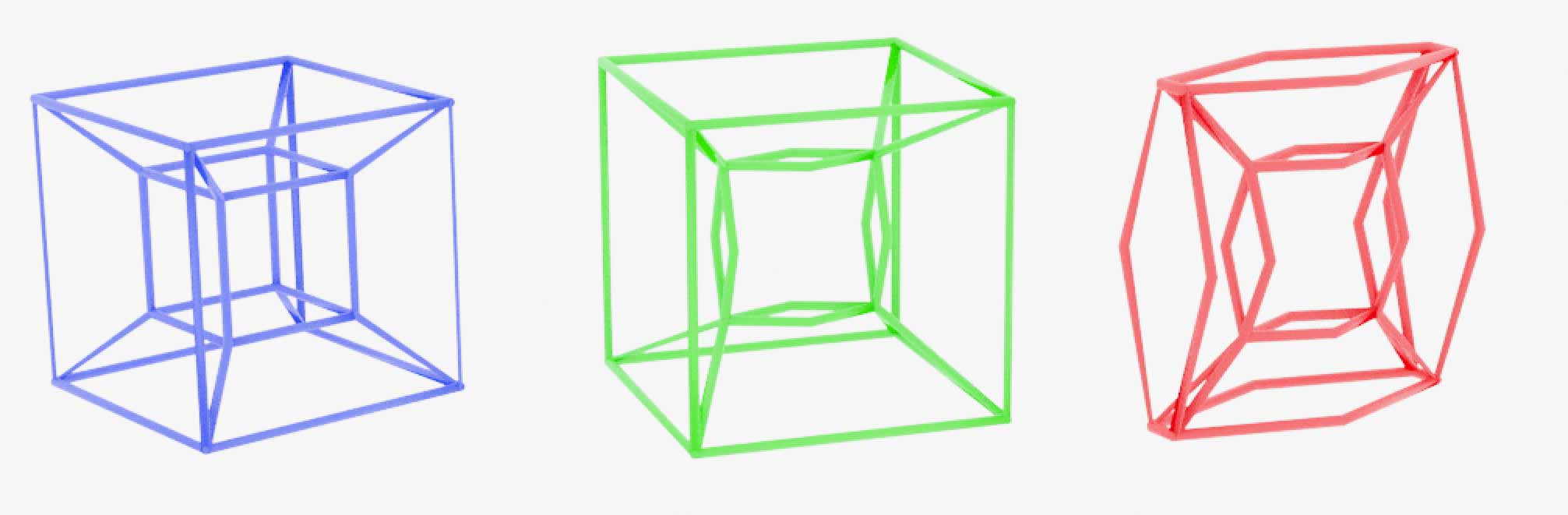
One-dimensional skeleton of a hypercube: A connected network of 32 edges, obviously $b_0=1$. We can count 17 holes in the 3D hypercube skeleton through homotopy transformation, i.e., $b_1=17$:

There’s actually a clever method to calculate the number of 1-dimensional loop holes $b_1$ for any graph. We first construct any tree (a graph with no loops) to cover all vertices. The number of edges not covered by the tree is the number of 1-dimensional loop holes. Because a loop-free tree is contractible to a point, the edges not covered by the tree become circles, and the entire graph is a wedge sum of those circles.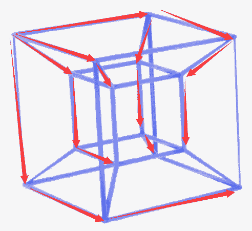
Two-dimensional skeleton of a hypercube: 24 square faces divide 3D space into 7 mutually disconnected cells. Note when counting the hypercube’s eight cells, we also count the large outer cubic cell. But in the homological sense, a 2-dimensional chain enclosing the large cubic cell can be obtained by adding seven 2-dimensional chains each enclosing one of the seven inner cells, so there are only 7 independent 2-dimensional holes, i.e., $b_2=7$. This shape is homotopy equivalent to a solid cube with seven bubbles inside. Bubbles cannot trap 1-dimensional loops, i.e., all 1-dimensional closed paths are contractible, so $b_0=1, b_1=0, b_2=7$.
On the n-dimensional sphere $S^n$, all spheres of dimension less than $n$ are contractible, so $b_0=1, b_1=b_2=…b_{n-1}=0, b_n=1$.
Since homotopy implies homology, n-dimensional space $\mathbb{R}^n$ and solid ball $D^n$ are both homotopy equivalent to a point, so Betti numbers are $b_0=1, b_1=b_2=…b_n=0$.
Sometimes homology groups cannot distinguish non-homotopic shapes. For example, the left figure below (wedge sum of two circles and a sphere) and the right torus both have 1 connected component, 2 one-dimensional holes, and one 2-dimensional hole: $b_0=1, b_1=2, b_2=1$. We’ll distinguish them later using cohomology theory.

Let’s look at homology groups of sphere-torus and torus-sphere: The sphere-torus’s longitude circles are non-contractible. Perpendicular to longitudes are meridian spheres - all meridians can contract to a point on the meridian sphere, but the 2D meridian sphere itself is non-contractible, so $b_0=1, b_1=1, b_2=1, b_3=1$. Actually torus-sphere is homeomorphic to sphere-torus - they interchange meridians and longitudes. That is, torus-sphere has non-contractible 1-dimensional meridian circles and non-contractible 2-dimensional spherical latitude surfaces, so the homology groups are the same.
Homology Groups of Product Spaces
Remember the product shapes mentioned in “4D Space (V): More Geometries [Part 1]“? Like the torus, sphere-torus and torus-sphere aren’t strictly geometric products but are topologically. Such topological spaces constructed through products are called product spaces. The Betti numbers of product space $A = B \times C$ are completely determined by those of $B$ and $C$, following the same pattern as coefficient changes after polynomial multiplication. For example, a torus is the product of two circles. A circle has Betti numbers $b_0=1, b_1=1$. Treating Betti numbers as coefficients to construct a polynomial $1+x$, the torus’s Betti numbers correspond to the polynomial $(1+x)(1+x) = 1+2x+x^2$. Extracting coefficients gives $b_0=1, b_1=2, b_2=1$. Why? Informally, after taking the product of two shapes, the homology chains also take products - an m-dimensional chain times an n-dimensional chain gives an (m+n)-dimensional chain. Finally adding up the quantities in each dimension naturally resembles polynomial multiplication with distribution then combining like terms. We can verify with torus-sphere (sphere-torus), which is the product of a circle ($b_0=1, b_1=1$, corresponding to polynomial $1+x$) and sphere ($b_0=1, b_1=0, b_2=1$, corresponding to polynomial $1+x^2$): $(1+x^2)(1+x) = 1+x+x^2+x^3$. The coefficients give $b_0=1, b_1=1, b_2=1, b_3=1$. With this theorem we can quickly calculate Betti numbers for torus-torus and double-torus, since they’re both homeomorphic to products of three circles. Since $(1+x)^3=1+3x+3x^2+x^3$, the Betti numbers at each order are $b_0=1, b_1=3, b_2=3, b_3=1$.
Generalization of Euler’s Formula: Euler-Poincaré Formula
Everyone should be familiar with Euler’s theorem for polyhedra: $V-E+F=2$. Rather than a theorem about polyhedra, this is really about graphs on spheres. If it’s not a sphere but a shape with $g$ holes, does Euler’s formula change? The answer is that Euler’s formula becomes $V-E+F=2-2g=\chi$. The number on the right is the Euler characteristic $\chi$. Generalizing to n dimensions, it’s the alternating sum of k-dimensional “face” counts $C_k$: $\chi=C_0-C_1+C_2-C_3+…C_n$. The Euler-Poincaré formula states that the Euler characteristic $\chi$ is a topological invariant equal to the alternating sum of the topological space’s Betti numbers at each dimension:
$\chi=C_0-C_1+C_2-C_3+…C_n=b_0-b_1+b_2-b_3+…b_n$.
This formula seems difficult to prove, but k-dimensional “face” counts $C_k$ and Betti numbers are actually degrees of freedom of certain groups. We just need to clarify their relationships. For triangulation, the number of vertices $C_0$ is exactly the degree of freedom of all zero-dimensional chain groups on the triangulation. Similarly, the number of edges $C_1$ is the degree of freedom of 1-dimensional chain groups, and the number of faces $C_2$ is the degree of freedom of 2-dimensional chain groups. Let’s see how homology group degrees of freedom arise: homology groups are quotient groups in the cycle group after viewing boundaries as equivalence classes. Denoting the degree of freedom of i-dimensional boundary groups as $B_i$ and i-dimensional cycle groups as $Z_i$, we have $Z_i=b_i+B_i$. What’s the relationship between cycle groups and general chain groups? If we view closed chains as “0” and construct a new equivalence class, then non-zero chains in this equivalence class are all non-closed (i.e., have boundaries) shapes. Two chains with the same boundary differ by a closed chain, so there are as many equivalence classes as different boundaries, i.e., $C_i=B_{i-1}+Z_i$. Combining the two equations gives $C_i=b_i+B_{i-1}+B_i$. Substituting all this into the left side of the equation to prove, noting that all 0-dimensional chains are cycles, i.e., the first term $C_0=Z_0=b_0+B_0$:
$C_0-C_1+C_2-…=(b_0+B_0)-(b_1+B_0+B_1)+(b_2+B_1+B_2)-…$
It’s easy to see on the right that all $B_i$ cancel out, leaving only the alternating sum of Betti numbers, proving the Euler-Poincaré formula. Through Betti numbers we can directly calculate Euler characteristics $\chi$ of various topological spaces without constructing specific triangulations.
Homology Groups of Non-orientable (One-sided) Surfaces
Let’s see if there’s anything special about homology groups of non-orientable one-sided surfaces like the Möbius strip, Klein bottle, and projective plane. The Möbius strip is actually homotopy equivalent to a circle, so there’s not much research value. The Klein bottle is a closed surface formed by gluing one pair of opposite edges of a rectangle directly and the other pair with a 180-degree twist like a Möbius strip. Here arrows indicate how rectangle edges are glued. The entire shape is connected, so obviously its zeroth homology group dimension $b_0=1$. For the first homology group, we have these candidate non-boundary chains: both red and blue paths should not be boundaries of any shape, because they feel non-contractible, but direct proof isn’t straightforward.
Let’s temporarily set aside the first homology group and see what the Klein bottle’s second homology group is. First we must find 2-dimensional cycles. But since the Klein bottle is non-orientable, we can’t cover the entire surface with consistently oriented triangles - we can’t find any 2-dimensional cycles. This will cause its second homology group order to be 0. Let’s try to verify:
- If we forcibly draw consistently oriented 2-dimensional chains inside the rectangle, the rectangle’s boundary won’t cancel but will double instead, so this 2-dimensional chain has a boundary and isn’t a cycle.

- If we start from the triangle in the upper left corner and gradually add triangles with the same orientation going right, note that when crossing the rectangle edge, orientation reverses according to the connection relationship between rectangle sides. In the end, the 2-dimensional chain we get still has a boundary.

Returning to the first homology group, we find these two double chains (brown in left figure and blue in right figure) are both boundaries: When we sew the surface, for general orientable surfaces, two circles have opposite directions and naturally cancel when overlapping, forming a shape with no boundary. But now due to opposite orientations on both sides, the boundary doesn’t disappear with sewing but doubles instead. This shows that twice the blue circle is indeed homologous to 0! A single blue circle in the right figure obviously isn’t the boundary of any shape. Addition of blue homology chains is special: like odd plus odd equals even, an even number of blue homology chains added equals 0, while an odd number added equals a single blue homology chain. Our homology group structure is no longer like integer addition but becomes the cyclic group of order 2, $C_2=\mathbb{Z}/2\mathbb{Z}$ - orientation is the culprit!
The dark yellow chain in the left figure has the same situation as the blue chain. Actually they’re homologous because they differ by a closed region $abchgc$ (readers please verify). In fact, both dark yellow and blue loops are meridians on the Klein bottle. These meridians can slide freely - they’re all homotopy equivalent.
However, the situation for latitudes is different. Since left and right sides must be glued with a twist, there are only two latitude lines parallel to the rectangle edges. Will two latitude loops be the boundary of some 2-dimensional chain and become 0? Actually not. If we try cutting along a latitude, the Klein bottle becomes a Möbius strip. On this non-orientable shape, we can’t find any 2-dimensional chain with only the Möbius strip’s boundary as its boundary. So overall, the Klein bottle’s first homology group consists of two parts: one infinite integer additive group and one finite modulo 2 integer additive group. The entire group is $\mathbb{Z}\times\mathbb{Z}/2\mathbb{Z}$. We say the Klein bottle has first Betti number $b_1=1$ plus a first torsion coefficient of 2.
Cohomology Theory
Let’s pause with homology examples and look at a new concept: cohomology. Chains can be added - can we further define multiplication between chains? It seems impossible directly, but we can define it through an algebraic “duality” method. We know numbers can certainly be multiplied. For distinction, let’s call the chains we discussed before chains and define a type of “cochains“ dual to chains - mappings that take general chains to numbers. This might make it convenient to define multiplicative structure between cochains. If readers haven’t encountered dual vector spaces, this might seem abstract. Figuratively, an n-dimensional cochain is a machine that takes in an n-dimensional chain and outputs a number. Different cochains are different machines. Looking at specific examples will clarify: the figure below shows a cochain mapping red and blue chains to two numbers respectively.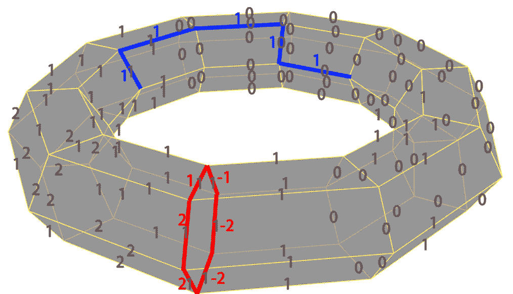
All gray numbers represent a 1-dimensional cochain: given any 1-dimensional chain, it can map it to a number by multiplying numbers at the same position by the chain’s multiplicity. For example, it maps the red chain above to $1\times 1+1\times (-1)+1\times (-2)+1\times (-2)+1\times 2+1\times 2=0$, and the blue chain to $1\times 1+1\times 1+1\times 0+1\times 0+1\times 0=2$.
Can mappings between chains correspond to cochains? This might allow us to directly transfer concepts like cycles and boundaries from chains. The answer is yes. Suppose mapping $f$ takes m-dimensional chain $a$ to n-dimensional chain $b$. If there’s an n-dimensional cochain $b’$ that can map n-dimensional chain $b$ to a number, since $b’(f(a)) = b’(b) = \text{a number}$, we find $b’(f(x))$ can map m-dimensional chain $x$ to a number, so this is actually an m-dimensional cochain, denoted $a’$. In other words, from the chain mapping $f$ we naturally induce a mapping between cochains $f’$, defined as $f’(b’)=a’$, with $f’(b’)(x)=a’(x)=b’(f(x))$. Note carefully that the induced mapping direction is reversed: $f$ goes from $a$ to $b$, while $f’$ goes from $b’$ to $a’$. This is a universal pattern between original spaces and dual spaces. These things are indeed convoluted - you can refer to my imaginative visualization of vector spaces and dual spaces - “Visiting the Infinite Pig Farm“ (warning: this is just a thought experiment that might make things more confusing).
Coboundary Operator
The boundary operator $\partial$ maps n-dimensional chains to (n-1)-dimensional chains. Correspondingly in cochains we can define the coboundary operator, which maps (n-1)-dimensional cochains to n-dimensional ones. If you’re still confused about these dual space concepts, this example should help: Find the coboundary of the 1-dimensional cochain marked with gray numbers and arrows on the triangulated annular shape below. According to our analysis, its coboundary should be a 2-dimensional cochain. The 2D face orientations are shown with arrows, so our task is to find the number on each 2D face.
For example, to find the number on the red triangle $ade$ at bottom left, how should we calculate? The coboundary mapping direction is opposite to chains, so we can construct a chain $ade$. Its boundary is $\partial(ade) = ad+de+ea$. This 2-dimensional coboundary will map the chain $ade$ to the same number that the original 1-dimensional cochain maps its boundary to, i.e., $1+4-6=-1$. Note the negative sign appears due to opposite direction. Similarly, numbers on other 2D faces can be obtained using algebraic sums of boundary numbers. For example, face $acd$ gets $-2$ because $2-3-1=-2$.
With concepts of cochains and coboundary operators, we’ll next define cocycles and coboundaries.
Cocycles
Cocycles require the coboundary of an n-dimensional cochain (which is (n+1)-dimensional!) to be 0. For example, the gray 1-dimensional cochain below is a cocycle - its coboundary is a 2-dimensional cochain that’s 0 everywhere (i.e., maps any 2-dimensional chain to 0).
From the figure above, we find that for the coboundary to be 0, the algebraic sum of numbers on each loop must be 0, i.e., cocycles map chains that are boundaries (i.e., these 1-dimensional chains are boundaries of some 2-dimensional chains) to 0. Note the middle $def$ is a hollow hole with no 2-dimensional chains on it. The 1-dimensional chain $de+ef+fd$ is just a cycle, not a boundary, so we don’t require cocycles to map it to 0.
Though this is intuitive, how do we prove this conclusion? If a chain is a boundary and doesn’t map to 0, by the definition of coboundary and boundary mapping relationships, the coboundary of the n-dimensional cochain would map the interior shape of the boundary to this same non-zero value - contradiction. If the chain isn’t a boundary, naturally we can’t find this chain’s “interior,” resulting in no (n+1)-dimensional chains at all, naturally equaling 0, so there’s no restriction on non-boundaries.
Coboundaries
Coboundaries require the n-dimensional cochain to be the boundary of some (n-1)-dimensional cochain. Again let’s translate this abstract language with a concrete example: the gray 1-dimensional cochain below is a coboundary because it’s the coboundary of the red zero-dimensional cochain.
Given an n-dimensional cochain, how do we determine if it’s a coboundary? Perhaps we can find that (n-1)-dimensional cochain: still using the 1-dimensional cochain above as example, let the zero-dimensional chain’s value at vertex $a$ be $x$. Since $\partial(ad) = a-d$ and the number marked on $ad$ is 1, we can deduce the zero-dimensional chain’s value at vertex $d$ is $x-1$. Calculating edge by edge this way, we can eventually construct the 0-dimensional cochain’s values at all vertices. However, if values at the same point derived through different paths differ, we have a contradiction - we can’t find the required zero-dimensional cochain, so that 1-dimensional cochain isn’t a coboundary. We find whether a 1-dimensional cochain is a coboundary depends on whether it has “path independence.” This path independence is equivalent to the cochain mapping the difference between two non-closed chains with the same start and end points to 0. These chains must be closed, so coboundaries must map all closed chains to 0 to ensure path independence. How do we prove this conclusion? An n-dimensional closed chain has no boundary. If the n-dimensional cochain doesn’t map it to 0, the (n-1)-dimensional cochain would map the closed chain’s boundary to this non-zero value, contradicting the fact that closed chains have no boundary.
Cohomology
Following homology chains, we construct cohomology equivalence classes through cocycles and coboundaries, thus constructing cohomology groups. Cocycles map all boundaries to zero, coboundaries map all cycles to zero. Note that boundaries are always cycles, so coboundaries mapping all cycles to zero also “incidentally” map all boundaries to zero. Therefore coboundaries are always cocycles, i.e., coboundaries are a subgroup of cocycles. If two cocycles differ by a coboundary, we say the two cocycles are cohomologous. Let’s look at this example specifically:
From the examples, we easily find that the two cohomologous cochains above both map chains homologous to $df+fe+ed$ to -1, i.e., those chains crossing the hollow hole $dfe$. Therefore cohomology groups also reflect information about holes in shapes, revealing a clever isomorphism between cohomology and homology groups. Here each cohomology class maps chains crossing the middle hole to different numbers. Addition between them is isomorphic to the integer additive group $\mathbb{Z}$. We can imagine if the shape has two holes, three holes, it would be $\mathbb{Z}^2$, $\mathbb{Z}^3$…
Actually at this point, we can use more vivid things to unveil cohomology’s mystery: it’s not hard to see that cocycles generally spread throughout the shape, and mappings that take chains to numbers are much like vector fields. Given a chain, the “flux” of the vector field (cochain) through this chain is a number. Cocycles are vector fields with no local vortices. Imagine a charge moving along a boundary in an electric field and returning to its starting point - the total work done is 0, ensuring local energy conservation. But if the charge runs around a hole along a meridian, energy increases - total energy isn’t conserved, so this field isn’t a coboundary. Cocycles require no vortices anywhere globally, so there can exist a “potential field” for the entire shape, ensuring global energy conservation. If a shape has holes, local energy conservation doesn’t guarantee global conservation - holes in the shape are exactly where non-conservation leaks through! Another example: in high school we learned about magnetic fields around current-carrying wires. The magnetic field outside the wire is (locally) irrotational, but the magnetic field around the wire has circulation proportional to current.
We’ve been discussing first cohomology groups. Let’s see what happens with zeroth cohomology groups: zero-dimensional cocycles map all zero-dimensional boundaries to zero. To satisfy this requirement, numbers marked at endpoints of each segment must be the same (think about why), i.e., vertices in the same connected component have the same marked numbers. Since all zero-dimensional chains are closed, coboundaries can only be 0-chains, i.e., the cohomology group is directly isomorphic to the cocycle group, which is isomorphic to the number of connected components. We can see that in this example, cohomology groups at each order are isomorphic to homology groups.
Introduction to de Rham Cohomology
If readers are familiar with multivariable calculus (skip this section if not), we can look at the relationship between Stokes’ theorem for vector fields and coboundary operators, answering what coboundary mappings correspond to in vector fields. Stokes’ theorem states that the integral of a vector field along a closed path equals the integral of the vector field’s curl through any surface bounded by that path. In plain language, the circulation of a vector field along a path equals the flux of the vector’s curl field through the loop. The surface bounded by the path is exactly a chain, its boundary is that path, naturally the vector field is a cochain, and the curl field of the vector field is that cochain’s coboundary. The coboundary operator is actually the n-dimensional generalization of gradient and curl operators - the exterior derivative operator!
Let’s look at some electromagnetic field examples: Generally, electric field $E$ has potential $\phi$ if the electric field is irrotational, i.e., from
$$\nabla \times E = 0$$
we can deduce there exists potential $\phi$ such that
$$\nabla \phi = E$$
However, this conclusion often fails. The reason we can happily use that conclusion much of the time is because field distributions often occupy simply connected regions without holes, where the first cohomology group is trivial. Now we know $\nabla \times E = 0$ means the electric field’s “coboundary” is 0, i.e., it’s a 1-dimensional cocycle. However, cocycles aren’t necessarily coboundaries unless the entire shape has no 1-dimensional holes. Let’s look at an example of first de Rham cohomology groups for vector fields on a torus. The meridian and latitude vector fields on the two tori below are both locally irrotational fields, but globally following the arrows around gives “net flux” - they’re generators of the first de Rham cohomology group. These electric fields definitely don’t have potential fields.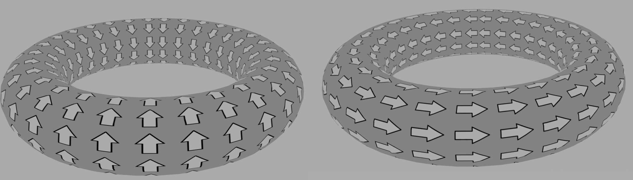
For example, the diagonal field on the torus below is also a locally irrotational field not cohomologous to 0. It’s obtained by superposing meridian and latitude fields.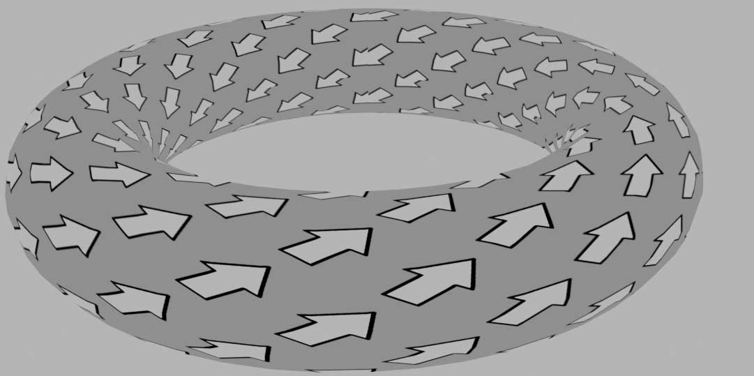
Since meridian and latitude fields can be freely superposed and combined, the entire group is $\mathbb{R}^2$. Note that previously we only considered integer coefficients for cohomology, yielding groups $\mathbb{Z}^2$. If we consider real coefficients, they’re all $\mathbb{R}^2$.
We see that specific “implementations” of cohomology and homology vary greatly, from intuitive chains to abstract cochain mappings, to even more abstract vector fields. Their “appearances” are completely different, but the resulting homology groups are the same. This shows homology isn’t specific to any particular implementation - like studying groups without caring about the meaning of specific elements, but abstracting out “homology axioms” described in the language of category theory, which we won’t expand on here.
Actually in field theory, fields $E$ satisfying $\nabla \times E = 0$ are called closed, corresponding to cocycles. Fields $E$ for which there exists $\phi$ such that $\nabla \phi = E$ are called exact, corresponding to coboundaries - just different customary names. That boundaries of boundaries are closed ($\partial^2=0$) corresponds to coboundaries of coboundaries being coclosed. This property becomes several versions in field theory depending on dimension: curl of gradient is 0, divergence of curl is 0… For higher-dimensional chains, we can use higher-dimensional n-vector fields (generally called differential form fields) as cochains. Through cohomology (i.e., finding fields with no local vortices but globally winding around higher-dimensional holes) we can discover higher-dimensional holes.
Cohomology Ring
Finally, let’s discuss how to multiply two cochains. If readers have read “4D Space (VII): N-Dimensional Vectors“, you know that at each point in a field, two m-vectors and n-vectors can yield an (m+n)-vector through wedge product. This gives us an (m+n)-vector field, i.e., an (m+n)-dimensional cochain. It can be proved that this multiplication is also well-defined between cohomology classes, meaning cohomology classes have not only addition but also multiplication. This algebraic structure with both addition and multiplication defined is called a ring, so cohomology is not just a group but a ring, with richer structure than homology groups.
For example, for the following two shapes, they have the same Betti numbers at each order (1,2,1 respectively), with identical homology groups at all dimensions. The two generators of the first cohomology group are marked in red and green. In the left figure, the two loops are disjoint - the cochains above have no common part when multiplied, yielding 0. In the right figure, meridian and latitude fields multiply to give a 2-dimensional vortex field over the entire torus, which is a basis for 2-dimensional cochains. Therefore the left and right figures have different cohomology ring structures, so they’re not homologous and therefore not homotopic.
Poincaré Duality
Have you noticed that many shapes’ Betti numbers at each order have a symmetry? For example, the n-dimensional sphere $S^n$ has $1,0,0,…,0,1$, the n-dimensional torus $T^n$ has binomial expansion coefficients $(1+x)^n$: $C_n^0,C_n^1,…,C_n^{n-1},C_n^n$, all symmetric. We call this Poincaré Duality. But the wedge sum of two circles is $1,2$, and the 2D annular region is $1,1,0$. The biggest difference between these two groups of shapes is that n-dimensional spheres and n-dimensional tori are all closed n-dimensional manifolds. Manifolds are generalizations of hypersurfaces: defined as topological spaces locally homeomorphic to flat space $\mathbb{R}^n$ - because smooth surfaces locally magnified all approximate planes. But at the wedge point of two circles, it’s no longer locally like a line ($\mathbb{R}$), and at the boundary of the 2D annular region, it’s no longer like a plane ($\mathbb{R}^2$), so they don’t have Poincaré duality.
Why do manifolds’ Betti numbers have duality? The answer is that triangulations on manifolds can be constructed to obtain dual triangulation structures. If readers are familiar with dual polyhedra and dual polytopes, you know that by selecting all face centers (cell centers) as vertices, we can construct new dual polyhedra (polytopes). This duality exactly corresponds i-dimensional shapes with (n-i)-dimensional shapes. This inspires us that for any triangulation, as long as we construct the dual triangulation, we can establish a correspondence from i-dimensional chain groups $C^i$ to (n-i)-dimensional cochain groups $C_{n-i}$. Why correspond chains to cochains? Because we can conveniently define cochains’ coboundaries, which correspond to chains’ boundary operations: a shape’s boundary is the sum of faces enclosing it, while a shape’s coboundary is the sum of all shapes having it as a face. As shown below, in the left figure $x$ as part of a 2-dimensional cochain, calculating the 1-dimensional cochain’s coboundary gives $x=a+b+c+d+e$. In the right figure $x$ as part of a zero-dimensional chain, calculating the 1-dimensional chain’s boundary gives $x=a+b+c+d+e$. Note that different triangulation methods don’t affect topological invariants, so homology groups calculated through dual triangulation must be the same as the original. We can deduce that i-dimensional chain groups $C^i$ are isomorphic to (n-i)-dimensional cochain groups $C_{n-i}$. Since coboundary operators on both sides also correspond, we can actually deduce that cohomology groups $H^i$ and $H_{n-i}$ are also isomorphic. Since cohomology and homology groups of the same order are isomorphic, after two group isomorphisms we finally get that two chain groups $H^i$ and $H^{n-i}$ are isomorphic, explaining the source of Betti number symmetry.
Actually we haven’t considered non-orientable manifolds here - their torsion coefficients don’t simply dualize. For specific details, please refer to formal algebraic topology textbooks.
Digression: Poincaré Conjecture and Poincaré Homology Sphere
Speaking of algebraic topology, probably few in the general public know about it, but the Poincaré conjecture in algebraic topology is quite famous. Poincaré’s conjecture is simple. Since an orientable n-dimensional connected closed topological space’s n-dimensional homology group must be $\mathbb{Z}$, and due to connectivity, the 0-dimensional homology group must also be $\mathbb{Z}$. If all other lower-dimensional homology groups are 0, this is the simplest kind of closed shape without holes. We should believe this n-dimensional space is an n-dimensional sphere. Poincaré conjectured that spaces with the same homology groups as spheres are only spheres, but he quickly found a counterexample. Poincaré constructed a “homology sphere” by gluing each face of a regular dodecahedron to its opposite face with a 1/10 twist (since opposite regular pentagons of a dodecahedron are exactly reversed, you can only twist by 1/10, 3/10, or 5/10 turns to glue them, yielding the Poincaré homology sphere, Seifert-Weber space, and real projective space respectively). It’s homologous to a normal 3-sphere but not homotopic, naturally not homeomorphic either.
Poincaré didn’t give up because of this counterexample. He revised the conjecture: if all paths on a closed surface are contractible, must it be a sphere? The answer is yes. With this restriction there are no more counterexamples, i.e., any simply connected, closed n-dimensional manifold must be homeomorphic to an n-dimensional sphere ($n \geq 2$). Mathematicians successively proved the Poincaré conjecture for higher-dimensional spheres, but the proof for this seemingly intuitive conclusion when $n=3$ was extraordinarily difficult, finally being solved by a Russian mathematician in 2006. Amazingly, his proof method not only solved Poincaré’s conjecture but also classified all 3-dimensional manifolds (which can be understood as curved cells). All 2-dimensional surfaces are classified by certain metric properties into spheres, planes, and hyperbolic spaces, while 3-dimensional space classification has eight types! Besides 3 types analogous from 2D to 3D and 2 product spaces, there are 3 anisotropic “strange spaces” where infinitely looping paradoxical staircases become possible… This is another wonderful story from geometric topology.