4D Space (XIII): Hyperspherical Harmonics
// This article only discusses solutions to certain partial differential equations on hyperspheres and does not involve imaginary 4D world physics settings, hence it is categorized in the 4D Space series.
// Note: This article contains many formulas. Feel free to ignore the details and just appreciate the various wave functions.
This time we’ll look at standing wave patterns on hyperspheres — what Hyperspherical Harmonics look like. They are solutions to the Laplace equation on hyperspheres and are related to possible wave function shapes of 4D atoms (which I plan to explore in detail in the next article). They can also accelerate 4D ray tracing rendering through “hyperspherical harmonic lighting” algorithms. Perhaps readers are already familiar with spherical harmonics on spheres and know that their expressions are somewhat complex. This article will try to avoid these complicated expressions and understand them from a new perspective.
2D “Circular Harmonics”
Following convention, let’s start with two dimensions. Imagine a circular thin membrane like a soap bubble that begins to deform and vibrate when subjected to external force (like flicking it with your finger). Simulating its vibration process is complex. Ignoring compression and stretching along the circumferential surface and considering only the spring-like restoring force in the perpendicular direction due to pressure differences, we obtain a second-order partial differential equation. The standard approach to solving it is called “separation of variables,” which intuitively decomposes arbitrary vibrations on the circle by frequency like a Fourier transform, finding several basic standing wave vibration modes (i.e., particular solutions to the equation). Any vibration under arbitrary conditions can be obtained by superposing these standing waves with different amplitudes.
The vibration modes on a circle are simple. Classified by the number of spatial vibration periods (also called angular quantum number), each class has two phase modes of sine and cosine vibrations. “Circular harmonics” are essentially trigonometric functions. These standing waves with different phases can be superposed to create traveling waves on the circle. Since these wave numbers coincide exactly with the quantum number concept in quantum mechanics, these period numbers are called angular quantum numbers.
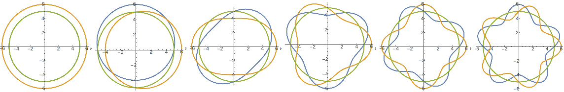
In summary, all vibration modes on a circle are:
| 0 | 1 | 2 | 3 | 4 | …… |
| $1$ | $\cos(\theta)$ | $\cos(2\theta)$ | $\cos(3\theta)$ | $\cos(4\theta)$ | …… |
| $\sin(\theta)$ | $\sin(2\theta)$ | $\sin(3\theta)$ | $\sin(4\theta)$ | …… |
Note that these standing wave functions are only amplitudes; actual motion requires multiplying by a time-dependent trigonometric function term. For example, angular quantum number 0 has only one “breathing” mode, corresponding to the soap bubble’s overall radial motion:
If a 2D “hydrogen atom” existed, according to the Schrödinger equation, its electron’s wave function distribution in the circumferential direction would match the standing waves on circles we analyzed, while the radial wave function would need to be solved based on the electron’s potential energy function. Together, the resulting wave functions would be similar to 3D atomic orbital shapes.
We won’t further analyze the electron’s 2D wave function here, but we can draw the following conclusions:
- The wave function’s total energy is quantized, called the principal quantum number $n$, which can take all natural numbers starting from 0.
- The wave function’s total angular momentum is also quantized, called the angular quantum number $l$, which can only take integers (positive/negative corresponding to clockwise/counterclockwise traveling waves), and limited by total energy must satisfy $-n \leq l \leq n$. Note that high total energy with small angular quantum number is allowed, indicating the wave function mainly vibrates in the radial direction.
3D Spherical Harmonics
The 3D problem becomes more complex. 2D vibrations only have radial and circumferential directions, described by two quantum numbers. 3D vibrations add another direction, requiring an additional quantum number. Solving after separation of variables in spherical coordinates encounters complex things like associated Legendre equations. In general: decompose the wave motion on a sphere into products and superpositions of longitudinal and latitudinal vibrations. Since longitude goes 360 degrees around, its vibration modes are the same as in two dimensions, taking all integers (positive/negative signs corresponding to sine/cosine phases). If we take the “north and south poles” as the $z$-axis, then vibrations along meridians represent rotation in the $xy$ plane, which can be interpreted as the angular momentum component in the $z$ direction, called the magnetic quantum number $m_l$. Vibrations along latitudes can have all natural number periods, but vibrations in this direction don’t have a good physical interpretation. We still prefer to use the angular quantum number $l$ corresponding to total angular momentum, i.e., the sum of meridional and latitudinal vibration numbers.

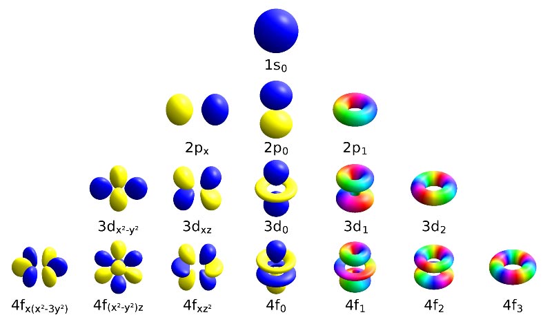
When I first studied chemistry in high school and saw these electron orbital shapes, I was puzzled: s-orbitals are spheres, p-orbitals are three perpendicular dumbbells, d-orbitals have 4 that are flower petals in different orientations, but why does one d-orbital have a stick with a hula hoop shape? Now the mystery is solved: the consistency of the previous orbital shapes was just coincidence—they’re all standing waves with different vibration frequencies in meridional and latitudinal directions that happen to look similar. (This coincidence has a reason—it reflects certain rotational properties of spherical harmonics)
Homogeneous Harmonic Polynomials (Solid Harmonics)
While we can qualitatively analyze standing wave patterns on circles and spheres, actually calculating spherical harmonic expressions is difficult. Before continuing to analyze 4D hyperspherical harmonics, let’s look at a new approach to handling spherical harmonics.
The difficulty in calculating spherical harmonics stems from restricting the wave equation to the sphere’s surface, where the Laplacian operator becomes very complex in spherical coordinates, making the equation hard to solve. The wave equation is actually simpler in Cartesian coordinates—just take second derivatives with respect to coordinates and add them up. If we ignore the spherical constraint and find special functions that permeate all of space, then restrict their domain to the sphere, we get Solid Harmonics. Don’t confuse these with hydrogen atom electron wave functions. Wave functions concentrate near the origin, while solid harmonics are polynomials that grow larger farther from the origin.
Specifically, we want to find spatial function fields $f(x,y,z)$ that don’t vary much radially (since we only care about the sphere), satisfying the Laplace equation—standing waves of the entire 3D space membrane vibrating in a fourth dimension. According to Taylor’s theorem, any function satisfying certain conditions can be approximated by polynomials, so we only need to consider polynomial solutions. Furthermore, since we want minimal radial variation, we prefer homogeneous polynomials. This way, when coordinates are all scaled radially by factor k, we can factor out the coefficient uniformly without causing different shapes of spherical harmonics at different radii. Thus our focus narrows to homogeneous harmonic polynomials, where harmonic means satisfying the Laplace equation $\partial^2 f/\partial x^2 + \partial^2 f/\partial y^2 + \partial^2 f/\partial z^2 = 0$. Let’s enumerate them by polynomial degree.
Constants (s orbitals)
Any constant has zero derivative, naturally satisfying the Laplace equation.
First-degree homogeneous polynomials (p orbitals)
While first-degree polynomials should be $f(x,y,z)=Ax+By+Cz+D$ and all satisfy the Laplace equation, the homogeneous condition requires no constant term, i.e., $f(x,y,z)=Ax+By+Cz$. This means $f_1=x$, $f_2=y$, $f_3=z$ can serve as “basis” functions to linearly combine all harmonic first-degree homogeneous polynomials. Restricting them to the sphere, they clearly correspond to the mutually perpendicular $p_x$, $p_y$, $p_z$ orbital spherical harmonics.
Second-degree homogeneous polynomials (d orbitals)
Second-degree homogeneous polynomials are $Ax^2+By^2+Cz^2+Dxy+Eyz+Fxz$, with six undetermined coefficients. For the Laplacian’s second derivative to be 0 requires $2A+2B+2C=0$, so there are actually only 5 degrees of freedom, matching the 5 d-orbitals. We can verify that $f_1=xy$, $f_2=yz$, $f_3=xz$ are three independent harmonic “basis” functions, while among $f_4=x^2-y^2$, $f_5=y^2-z^2$, $f_6=x^2-z^2$ only two are linearly independent. Though we could choose any two, to match the classification by z-axis angular momentum, we symmetrically choose $f_4$ and $f_5+f_6$. This choice isn’t unique—it just gives basis standing waves with nodal lines in meridional and latitudinal directions, best matching their quantum number descriptions. It’s like shooting the spherical harmonic arrow first then painting the homogeneous polynomial target. Actually, the $z$-axis isn’t special at all—we could choose the $x$-axis as the sphere’s poles with the $yz$ plane as the equator, and still linearly combine all the spherical harmonic bases from those obtained with $z$-axis poles.
Observing the number of wave peaks in meridional and latitudinal directions for these functions, we can determine their quantum numbers. Organizing these harmonic homogeneous polynomials gives us this table:
| J\Jz | -2 | -1 | 0 | 1 | 2 |
| 0 | $1$ | ||||
| 1 | $x$ | $z$ | $y$ | ||
| 2 | $xy$ | $xz$ | $x^2+y^2$$-2z^2$ | $yz$ | $x^2-y^2$ |

Note: Some details we haven’t covered:
- While the polynomials in the table are orthogonal in standard function space, they’re not normalized—the true basis functions need to be multiplied by some ugly coefficients, which I’ve omitted for simplicity.
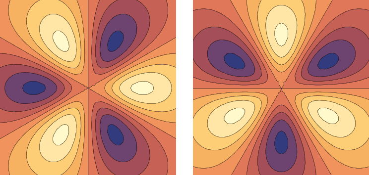
- Quantum mechanics conventionally uses complex spherical harmonics. For example, p-orbitals don’t choose bases $x$, $y$, $z$, but rather $x+iy$, $x-iy$, $z$, because the latter are common eigenstates of angular momentum and z-axis angular momentum component. They can be viewed as traveling waves rotating around the $z$-axis formed by superposing standing waves of different phases, so amplitude is uniform everywhere while phase (hue) varies with rotation angle, looking like donuts.
4D Hyperspherical Harmonics
Even if you don’t know how to solve partial differential equations or understand group representation theory, using solid harmonic techniques we can roughly determine the distribution of 4D hyperspherical harmonics and their quantum numbers. How should we choose quantum numbers? The simplest idea is: since we already know vibration modes on spheres, we can add another directional vibration through hyperspherical coordinates. Hyperspherical coordinates determine positions on hyperspheres like this: given a primary latitude determining a latitude hypersphere (like a latitude circle), then use regular spherical coordinates with secondary latitude and longitude to finally determine the point. Hyperspherical harmonic quantum numbers can use the same approach: first take the $w$-axis as the north-south pole direction, count waves in the $w$ direction, then look at total waves on the $xyz$ sphere, which subdivides like spherical harmonics into two steps: waves in the $xy$ plane, and remaining waves in the $z$ direction.
s orbitals (total angular quantum number 0):
Only the constant term, no spatial wave fluctuations. Both quantum numbers are 0, which we put in this table:
| Mxyz\Mxy | 0 |
| 0 | 1 |
p orbitals (total angular quantum number 1):
Also simple—four coordinate axes correspond to four bases. We count their spatial period quantum numbers and fill this table:
| Mxyz\Mxy | -1 | 0 | 1 |
| 0 | $w$ | ||
| 1 | $x$ | $z$ | $y$ |
d orbitals (total angular quantum number 2):
First we want a standing wave vibrating entirely in the $w$ direction, but $w^2$ alone has Laplacian value 2. To cancel it, we can add an isotropic term $r^2=x^2+y^2+z^2$ with no fluctuations in the $xyz$ cell. You can verify that $x^2+y^2+z^2-3w^2$ is harmonic. Then we continue finding terms with only one wave in the $w$ direction, i.e., terms with $w$ to the first power. We can obviously find three: $xw$, $yw$, $zw$. Finally, for no vibration in the $w$ direction, we directly bring over spherical harmonic expressions without $w$, filling this table:
| Mxyz\Mxy | -2 | -1 | 0 | 1 | 2 |
| 0 | $x^2+y^2+z^2-3w^2$ | ||||
| 1 | $xw$ | $zw$ | $yw$ | ||
| 2 | $xy$ | $xz$ | $x^2+y^2-2z^2$ | $yz$ | $x^2-y^2$ |
f orbitals (total angular quantum number 3):
Similar approach to d orbitals. First we want a standing wave vibrating entirely in the $w$ direction, but $w^3$ alone has Laplacian value $6w$. To cancel it, we can add an isotropic term $r^2w=(x^2+y^2+z^2)w$ with no fluctuations in the $xyz$ cell. You can verify that $(x^2+y^2+z^2)w-w^3$ is harmonic. Then we continue finding terms with two waves in the $w$ direction, i.e., $w$ squared terms like $xw^2$, but it’s not harmonic by itself and needs matching terms like before, yielding $x^3-3xw^2$ as harmonic. Similarly we can find two other harmonic functions along $y$ and $z$ axes. Then for $w$ to the first power terms, the previous examples suggest we might directly multiply spherical harmonic d-orbital polynomials by $w$, and calculation shows they indeed remain harmonic. Finally, for no vibration in the $w$ direction, we directly bring over spherical harmonic f-orbital expressions, getting this table. (Friendly reminder: this table doesn’t display completely on mobile portrait mode—please view in landscape.)
| Mxyz\Mxy | -3 | -2 | -1 | 0 | 1 | 2 | 3 |
| 0 | $(x^2+y^2+z^2)w-w^3$ | ||||||
| 1 | $x^3-3xw^2$ | $z^3-3zw^2$ | $y^3-3yw^2$ | ||||
| 2 | $xyw$ | $xzw$ | $(x^2+y^2-2z^2)w$ | $yzw$ | $x^2w-y^2w$ | ||
| 3 | $x^3-3xy^2$ | $xyz$ | $(x^2+y^2-4z^2)x$ | $(x^2+y^2-\frac{2}{3}z^2)z$ | $(x^2+y^2-4z^2)y$ | $x^2z-y^2z$ | $y^3-3x^2y$ |
Hyperspherical Harmonics in Hopf Coordinates
Since 4D space’s double rotation effect means $xy$ and $zw$ planes don’t interfere, why not choose the angular momenta in these two planes as quantum numbers, i.e., count wave oscillations in the $xy$ plane and $zw$ plane separately? This approach corresponds to using another 4D polar coordinate system—Hopf coordinates. We’ve already analyzed its advantages over the other hyperspherical coordinates. What differences will hyperspherical harmonics have in this coordinate system? As a reminder, starting in four dimensions we must use the direction of the angular velocity bivector, not the stationary rotation axis direction, to describe rotation. For example, $J_{xy}=1$ represents waves in the $xy$ plane, corresponding to rotation occurring in the $xy$ plane, with the $zw$ plane being the stationary rotation “axis.”
s orbitals (angular quantum number 0):
Only the constant term, no spatial wave fluctuations. Both quantum numbers are 0, which we put in this table:
| Jxy\Jzw | 0 |
| 0 | 1 |
p orbitals (angular quantum number 1):
Also simple—four coordinate axes correspond to four bases. We count their spatial period quantum numbers and fill this table:
| Jxy\Jzw | -1 | 0 | 1 |
| -1 | $x$ | ||
| 0 | $z$ | $w$ | |
| 1 | $y$ |
d orbitals (angular quantum number 2):
Products of two coordinates are all harmonic (satisfy the Laplace equation), giving us 6 candidate bases: $xy$, $xz$, $xw$, $yz$, $yw$, $zw$. Additionally, observing that $(x^2)’’=2$, such squared terms must appear in pairs to cancel each other for harmonicity, i.e., $x^2-y^2$, $x^2-z^2$, $x^2-w^2$, $y^2-z^2$, $y^2-w^2$, $z^2-w^2$ as 6 candidate bases. Similar to 3D, we find three of these six bases are linearly dependent. How to choose? Since we selected wave numbers in the $xy$ and $zw$ planes as quantum numbers, we prioritize keeping $x^2-y^2$ and $z^2-w^2$. For the third, we see that all previously selected bases have waves in xy or zw, i.e., the east-west and yin-yang longitude directions in 4D hypersphere Hopf coordinates. Using those bases we can superpose a wave function vibrating only in the north-south direction (vibrating between $xy$ and $zw$ planes): $x^2+y^2-z^2-w^2$, which is our final basis. Counting by quantum numbers gives this table:
| Jxy\Jzw | -2 | -1 | 0 | 1 | 2 |
| -2 | $x y$ | ||||
| -1 | $xz$ | $xw$ | |||
| 0 | $zw$ | $x^2+y^2-$$z^2-w^2$ | $z^2-$$w^2$ | ||
| 1 | $yz$ | $yw$ | |||
| 2 | $x^2-y^2$ |
f orbitals (angular quantum number 3):
Getting intense now. Through various techniques (using orthogonality conditions with undetermined coefficients, etc.) we can derive the results in the table below. Here $C = 3(x^2+y^2-z^2-w^2)$. Friendly reminder: this table doesn’t display completely on mobile portrait mode—please view in landscape.
| Jxy\Jzw | -3 | -2 | -1 | 0 | 1 | 2 | 3 |
| -3 | $x^3-$$3xy^2$ | ||||||
| -2 | $xyz$ | $xyw$ | |||||
| -1 | $xzw$ | $x(C-2x^2)+$$\frac{5}{9}(x^3-3x y^2)$ | $xz^2-$$xw^2$ | ||||
| 0 | $z^3-$$3zw^2$ | $\frac{5}{9}(z^3-3z w^2)$$-z(C+2z^2)$ | $\frac{5}{9}(w^3-3z^2w)$$-w(C+2w^2)$ | $w^3-$$3z^2w$ | |||
| 1 | $yzw$ | $y(C-2y^2)+$$\frac{5}{9}(y^3-3x^2y)$ | $yz^2-$$yw^2$ | ||||
| 2 | $x^2z-$$y^2z$ | $x^2w-$$y^2w$ | |||||
| 3 | $y^3-$$3x^2y$ |
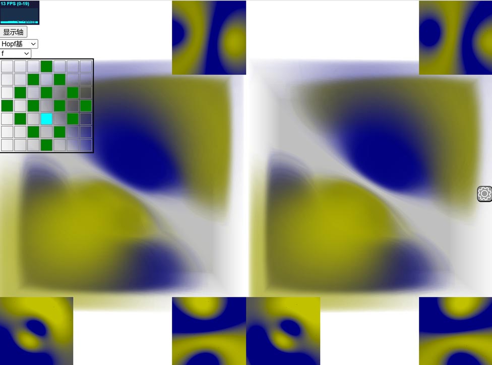
Can’t intuitively imagine these function shapes from the expressions? I’ve prepared a corresponding scene in Tesserxel. With display axes enabled, the scene marks where the x, y, z, w axes pierce the hypersphere with colors.
Isoclinic Double Rotation Waves
Did you notice that these tables all have diamond-shaped arrangements? This suggests if we do a variable substitution $J^{+}=J_{xy}+J_{zw}$, $J^{-}=J_{xy}-J_{zw}$, we can rotate the table 45 degrees to make it more compact. However, when the total angular quantum number is odd, both quantum numbers $J^{+}$ and $J^{-}$ can only take odd values, while for even total angular quantum numbers, both can only take even values. We conventionally divide them by two, becoming integers and half-integers, somewhat reminiscent of electron spin quantum numbers.
s orbitals:
| J+\J- | 0 |
| 0 | 1 |
p orbitals:
| J+\J- | -1/2 | 1/2 |
| -1/2 | $x$ | $z$ |
| 1/2 | $w$ | $y$ |
d orbitals:
| J+\J- | -1 | 0 | 1 |
| -1 | $xy$ | $xz$ | $zw$ |
| 0 | $xw$ | $x^2+y^2-z^2-w^2$ | $yz$ |
| 1 | $z^2-w^2$ | $yw$ | $x^2-y^2$ |
f orbitals:
| J+\J- | -3/2 | -1/2 | 1/2 | 3/2 |
| -3/2 | $x^3-3xy^2$ | $xyz$ | $xzw$ | $z^3-3zw^2$ |
| -1/2 | $xyw$ | $x(C-2x^2)+$$\frac{5}{9}(x^3-3xy^2)$ | $\frac{5}{9}(z^3-3zw^2)$$-z(C+2z^2)$ | $yzw$ |
| 1/2 | $xz^2-xw^2$ | $\frac{5}{9}(w^3-3z^2w)$$-w(C+2w^2)$ | $y(C-2y^2)+$$\frac{5}{9}(y^3-3x^2y)$ | $x^2z-y^2z$ |
| 3/2 | $w^3-3z^2w$ | $yz^2-yw^2$ | $x^2w-y^2w$ | $y^3-3x^2y$ |
This is no coincidence—the group structure of 4D rotations explains this phenomenon well: 4D rotations can be uniquely decomposed into superpositions of left and right isoclinic rotations, i.e., the direct product of left and right isoclinic rotation groups is a double cover of the 4D rotation group, and each isoclinic rotation group is isomorphic to the double cover of the 3D rotation group, i.e., the spin group.
One thing is quite strange: although left and right isoclinic rotation components $J^+$ and $J^-$ don’t interfere and can have definite left and right rotation quantum numbers simultaneously, the bases in the tables above have equal total left and right isoclinic rotation magnitudes $J_L^2$ and $J_R^2$, producing only simple rotations. ($J^+$ is just one of the three components of $J_L$, like the relationship between $J_z$ and $J$ in 3D space; similarly $J^-$ is one of the three components of $J_R$.) Expanding the calculation shows that the operator reflecting bivector singularity simplifies to 0, i.e., $J\wedge J=2(J_{xy}J_{zw}-J_{xz}J_{yw}+J_{xw}J_{yz})=0$, which further gives $J_L^2=J_R^2$ always holds, meaning no wave phenomena related to double rotations exist. You might ask: can’t I superpose angular momentum eigenstates in the xy and zw planes separately to get a double rotation state? Calculation shows that while such a superposition state has $J^+$ and $J^-$ with one greater than 0 and one equal to 0, these are just components of left and right isoclinic rotations—$J_L^2$ and $J_R^2$ are still equal.
Why are there no double rotation wave functions? My personal understanding is: since isoclinic double rotation trajectories on hyperspheres form the Hopf fibration, if such traveling waves existed, they would only change phase along Hopf fibers with no waves in other directions. Constructing such functions would be equivalent to describing any point on the hypersphere directly by its phase and which fiber it’s on, essentially mapping the hypersphere $\mathrm S^3$ one-to-one onto the non-homeomorphic $\mathrm S^2\times \mathrm S^1$. In other words, there would exist wavefronts of constant phase on the Hopf fibration, but the Hopf fibration has no such global section structure.
Highly Symmetric Standing Waves
The spherical and hyperspherical harmonics we’ve seen were divided by meridians and latitudes in various polar coordinates for computational convenience. Are there waves with better symmetry? For example, do hydrogen atomic orbitals with dodecahedral symmetry exist? Science fiction writer and amateur mathematician Greg Egan provides the answer on his website: Since spherical harmonics are complete, we can use them like Fourier series to synthesize any other function, so the dodecahedral symmetric waves we seek are still composed of those general spherical standing waves. Greg Egan’s idea is simple: first take any wave, then apply all the dodecahedron’s symmetry rotation operations to it, and the superposition will certainly have dodecahedral symmetry. However, often such superposition causes all waves to cancel, giving 0. Only for certain angular quantum number values do we get non-zero solutions. For example, when ℓ = 0, 6, 10, 12, 15, 16, 18, 20, 21, 22, 24, 25, 26, 27, 28, 31, 32, 33, 34, 35, 37, 38, 39, 41, 43, 44, 47, 49, 53, 59… there’s one non-zero solution, while for ℓ = 30, 36, 40, 42, 45, 46, 48, 50, 51, 52, 54, 55, 56, 57, 58, 61, 62, 63, 64, 65, 67, 68, 69, 71, 73, 74, 77, 79, 83, 89… there are two linearly independent solutions. The patterns are explained on his website.
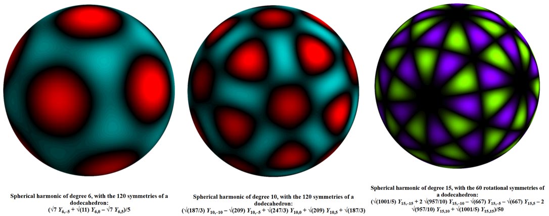
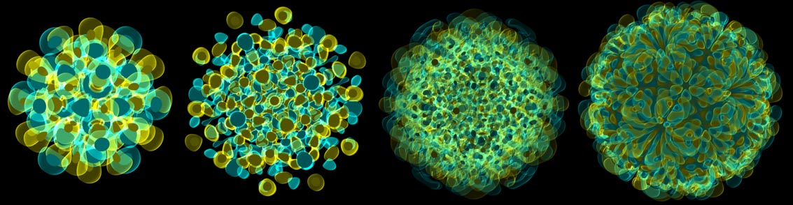
Greg Egan didn’t stop at three dimensions—he used similar methods to find standing waves on hyperspheres with 120/600-cell symmetry. Stereographically projecting the hypersphere down and marking the wave function’s equal-amplitude surfaces produces the structures below.
Applications of Hyperspherical Harmonics
Finally, let’s discuss some practical uses of hyperspherical harmonics. Like Fourier series and spherical harmonics, they form a complete orthogonal basis for functions on hyperspheres, allowing compression and storage of global illumination information in 4D scene rendering through methods similar to 3D. For an explanation of the principles of 3D spherical harmonic lighting, see this video course “GAMES202-High Quality Real-time Rendering”(In Chinese).
Additionally, while 4D hyperspherical harmonics exceed our real 3D space and seem impractical, when solving multi-quantum problems in the 3D world, their wave functions exist in spaces with dimensions greater than three. This is where 4D and higher hyperspherical harmonics become useful—see books like “Hyperspherical Harmonics and Their Physical Applications.”
References
[1] Harmonic polynomials, hyperspherical harmonics, and atomic spectra
This paper describes constructing hyperspherical harmonics through harmonic polynomials and derives that the eigenvalue of the angular momentum squared operator in $d$ dimensions is $l(l+d-2)$, where $l$ is the angular quantum number.
[2] Hyperspherical harmonics with arbitrary arguments
This paper describes hyperspherical harmonics in two 4D polar coordinates and gives the correspondence between their quantum numbers.
[3] Greg Egan. Symmetric Waves
Greg Egan’s original website article.