4D Computer Graphics: Rendering

Previous articles have covered almost all common methods for visualizing 4D: cross-section method, stereographic projection, contour surfaces or color-coding the fourth dimension, 3D photos, etc. Among these, 3D photos are further divided into wireframe and voxel cloud display methods. While most readers can probably understand these methods, implementing them in computer programs is quite a challenge. Here I’ll first introduce some basic computer graphics principles, then delve into various methods for rendering complex 4D objects. Readers can choose sections based on their knowledge level. Perhaps I’ll start a series later specifically explaining how to build a 4D graphics engine step by step.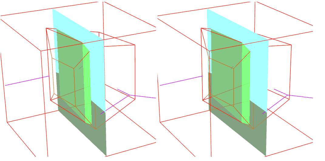

Featured Content

• 3D Computer Graphics Fundamentals
• Voxel/Cross-section 4D Graphics Rendering
  • Shadertoy Online 4D Path Tracing Demo
  • Tetrahedron Method/Cell Complex Method
  • Voxel Cloud Rendering Methods
• Wireframe Rendering Occlusion Culling Algorithm

Computer Graphics Fundamentals

Let me first briefly introduce the basics of 3D computer graphics. If you’re already very familiar with this content, please skip to the next section. For those wanting to learn more, there are abundant online tutorial resources. I particularly recommend this online course: “GAMES101-Introduction to Modern Computer Graphics-Lingqi Yan”.

How do computers display graphics? A monitor is essentially a bunch of neatly arranged colored lights emitting different proportional intensities. Graphics are fundamentally a 2D pixel array storing numbers representing these light emission intensity ratios. To quickly calculate these pixels numbering in the hundreds of thousands or millions, GPUs (Graphics Processing Units) were invented. Unlike CPUs that execute one instruction at a time, GPUs receive one instruction and simultaneously perform the same operation on all pixels, making parallel computation thousands of times faster than CPUs processing one pixel at a time.

1. Rasterization Technology

How do GPUs calculate and display 3D graphics? The mainstream approach only draws three basic primitives: points, lines, and triangles. The hardware is specifically optimized for drawing these primitives, allowing very fast operation. Here’s the general process for drawing triangles: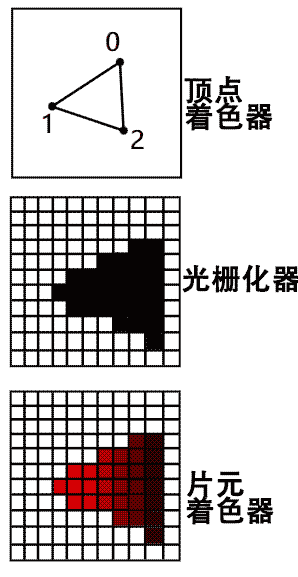

1. First, send the vertex data of triangles composing the geometry to the GPU
2. In the GPU, perform coordinate transformations on all vertex data in parallel to get the final perspective projection coordinates in the image. This vertex coordinate transformation program is called the “Vertex Shader“
3. Through the hardware-optimized “Rasterizer“, quickly determine which pixels belong to the triangle’s interior and calculate their barycentric coordinates relative to the triangle. This part of the program is hardcoded in hardware and generally not programmable.
4. Color all pixels determined to be inside the triangle in the previous step. This program is called the “Fragment Shader“. Note that these pixels can be differentiated based on barycentric coordinate information to be colored differently, such as mapping to various textures to achieve many material detail effects.

Rasterization has some non-trivial details, such as view frustum culling in the rasterizer stage and occlusion culling in the fragment shader stage.

View Frustum Culling

Our earlier statement that the vertex shader outputs projected coordinates on the screen is actually inaccurate, because direct rendering has serious problems. Imagine a camera at the origin with a projection canvas at $z=1$. Using triangle similarity or solving line equations, the position of a distant point $p(x,y,z)$ on the canvas is $b(x/z,y/z,1)$.This $1/z$ factor causes the most important perspective phenomenon of “objects appear smaller when farther away”, so this division by $z$ is called “perspective division”. However, perspective division brings a serious problem: points behind the camera will appear in front of it. For example, points $p(x,y,z)$ and $p(-x,-y,-z)$ both map to the same point $(x/z,y/z)$ on the screen, but actually only the point in front of the camera can be seen. Therefore, we need to introduce view frustum culling, which must be completed before perspective division. The view frustum is a virtual pyramid representing the camera’s field of view in the scene. Objects outside the frustum won’t be rendered. Traditional GPUs combine projection transformation with view frustum culling using a mathematical tool called “Homogeneous Coordinates“.

Since we can’t divide by the factor $z$ early, it’s specified that vertex shaders need to output “homogeneous coordinates”. These coordinates treat all parallel vectors as identical, i.e., points $(x,y,z)$, $(kx,ky,kz)$, and $(x/z,y/z,1)$ all correspond to the same point $(x/z,y/z)$ on the canvas. But the graphics card only renders points where the third component of homogeneous coordinates is greater than 0, thus avoiding rendering objects behind the camera. Homogeneous coordinates not only linearize the non-linear perspective transformation but also easily handle view frustum culling. Note that view frustum culling cannot be completed solely in the vertex shader stage; it continues in the rasterization stage for each pixel, otherwise you can’t correctly render line segments or triangles that are partially in front of and partially behind the camera.

Occlusion Culling

Besides culling objects behind the camera, we also need to cull objects occluded by foreground objects. The simplest idea (called the painter’s algorithm) is to sort objects by distance from camera and render from far to near, with later colors automatically covering earlier ones. But pre-sorting is cumbersome and may encounter mutual occlusion problems between objects, so this fixed drawing order method is not feasible.In mature 3D rendering pipelines, occlusion culling uses z-depth buffer technology. When drawing each primitive, besides executing the fragment shader to color pixels, it also renders a grayscale image containing only z-axis depth information, called the “Depth Buffer”. When drawing a pixel of the next primitive, it compares with the depth value in the depth buffer. If the depth buffer’s depth is closer, it means this pixel is behind the previously drawn pixel, so coloring is abandoned. The previous homogeneous coordinates happen to retain $z$-axis depth information before perspective division - can we use it directly for the depth buffer? No. Computer number storage precision is limited. Objects can be very close or far from the camera, and near details are often more important than distant ones, requiring more precision. So rather than storing depth value $z$, it’s more economical to store its reciprocal $1/z$.

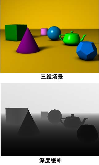
Now we need both occlusion culling and homogeneous coordinates for view frustum culling. It’s specified that the vertex shader’s final output is a 4D homogeneous coordinate vector: the first two components for screen position, the third for depth testing, and the fourth for perspective division. For example, a point $(x,y,z)$ in space becomes $(x,y,1,z)$, and after perspective division becomes $(x/z,y/z,1/z,1)$, achieving camera back-face culling, correct perspective scaling, and non-uniform precision depth buffering. Actually, all data needing interpolation inside triangles (like texture coordinates) must be completed before perspective division, otherwise it causes perspective distortion like the left texture below.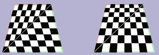In summary, while you might think the vertex shader only outputs 2D point coordinates on screen, it’s actually a 4D homogeneous coordinate, which is very necessary!

2. Ray Tracing Technology

The advantage of rasterization is speed and mature technology, but since drawing triangles differs from real optical imaging processes, implementing complex shadows, refraction, reflection and other optical phenomena becomes very difficult (you should have experienced some of this with view frustum culling and occlusion culling). Thus another method was born - ray tracing. Cameras can photograph objects because photosensitive devices behind the lens receive light rays. The most naive approach is to have light sources in the scene uniformly sample and randomly emit photons, simulate light bouncing, and if they hit a pixel’s “photosensitive area” in the camera, record that photon’s contribution to color brightness. However, this algorithm is very inefficient because camera photosensitive areas are generally small, and many photons ultimately won’t reflect into the lens. A simple scene might need hundreds of millions of photons to barely get a viewable photo.

The solution is simple. Since light paths are reversible, we can uniformly sample and randomly emit rays from the camera to bounce off objects. As long as they hit a light source, we can work backwards to find that ray’s brightness contribution. This is the simplest path tracing rendering method, capable of rendering photographic quality images! Of course, it also needs many rays, especially when light sources are small, the probability of hitting them is also very small. This simulation of random light bouncing has a side effect of producing many noise spots in the image. To reduce noise, you can only increase the number of sampled rays per pixel.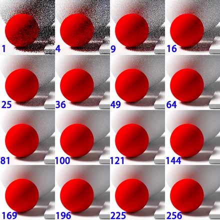

Actually, if photographic realism isn’t required, we can stop when hitting the first diffuse object surface and directly calculate that pixel’s color based on the object’s diffuse color (like Lambert, Phong lighting models), rather than continuously randomly reflecting and tracing to the illuminating light source. This avoids noise and the need to sample many rays, computing much faster, though lacking multiple light bounces makes objects look much less realistic.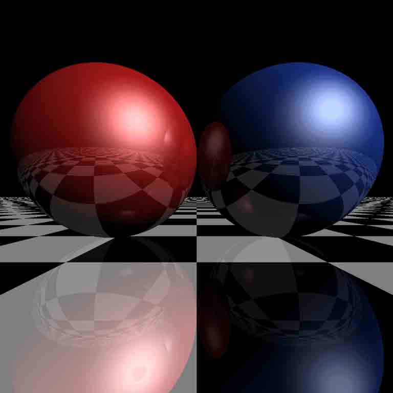

How specifically to use GPU for ray tracing? We can cover the entire image with two triangles, disguising it as rasterization rendering for the GPU, and calculate ray-object intersections, colors, etc. in the fragment shader code that colors each pixel. But GPUs can only quickly execute the same instructions in batches. Whether rays intersect objects makes subsequent commands very different for different pixels, greatly reducing ray tracing’s parallel computing efficiency on GPUs, so ray tracing is much slower than rasterization. To solve this problem, people designed hardware ray tracing that can quickly handle batch triangle intersections (like Nvidia’s RTX series).

4D Scene Rendering Methods

That’s the basics of 3D computer graphics. Now we can finally formally introduce 4D computer graphics. Unlike 3D, before studying 4D graphics rendering algorithms, we must first determine methods for visualizing 4D graphics. Below I’ll introduce the most widely used cross-section method and my favorite voxel method.

1. Voxel/Cross-section Rendering

Compared to 3D, the biggest difference in 4D scene rendering is that the image itself becomes a 3D array. Besides dimensionality, there’s no essential difference. To run on GPUs, we need to layer the 3D array and have the GPU process each layer to get ordinary 2D images - that’s cross-section rendering. Both rasterization and ray tracing technologies can accomplish this task.

1.1 Ray Tracing

4D ray tracing is almost identical to 3D. I recommend first familiarizing yourself with how simple 3D ray tracing fragment shaders are written. I recommend Shadertoy, a website where you can edit online and browse shaders written by various experts.

Common shader languages (GLSL/WSL/HLSL) support the vec4 type for 4D vectors. Although designed for representing 3D homogeneous coordinates or RGBA color components, this conveniently allows us to represent 4D coordinates. The most important thing in ray tracing is calculating ray-object intersections. If we only consider intersections with planes and spheres, we just need to change vec3 to vec4 in normal ray tracing code, fill the fourth dimension with 0, and directly upgrade the scene to intersect with hyperplanes and hyperspheres!

Below is a real-time path tracing scene I randomly found on Shadertoy: Since it generally loads very slowly on mobile browsers, please click the image below carefully to activate: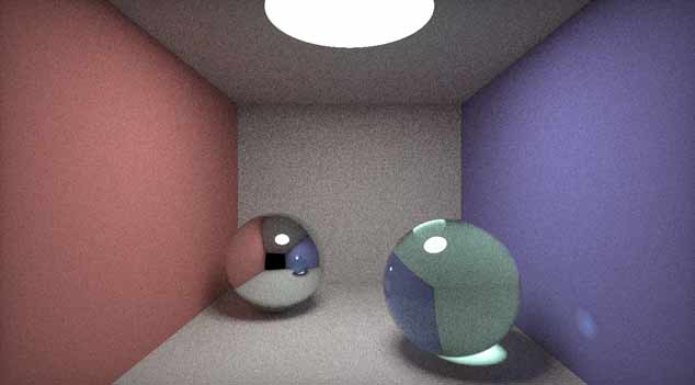

How to make this 3D scene 4D? First I replaced all vec3 with vec4, then since path tracing encounters uniform random sampling on hypersphere surfaces, I needed to modify the sampling formula. Click here to expand pseudocode for generating uniformly distributed unit 3D and 4D vectors.

function generateRandVec3(){
  let a = Math.random() * 2.0 * Math.PI;
  let c = Math.random() * 2.0 - 1.0;
  let b = Math.sqrt(1.0 - c * c);
  return new Vec3(b * Math.cos(a), b * Math.sin(a), c);
}
function generateRandVec4(){
  let a = Math.random() * 2.0 * Math.PI;
  let b = Math.random() * 2.0 * Math.PI;
  let c = Math.random();
  let sc = Math.sqrt(c);
  let cc = Math.sqrt(1.0 - c);
  return new Vec4(sc * Math.cos(a), sc * Math.sin(a), cc * Math.cos(b), cc * Math.sin(b));
}

I replaced the sphere uniform sampling formula with hypersphere sampling, added walls and two hyperspheres in the fourth dimension, then set mouse left-right drag to rotate camera, up-down drag to translate the cross-section position in the fourth dimension. This 4D scene demo is transformation complete(four-directional attack)! Tip: Click the image below to activate the scene.

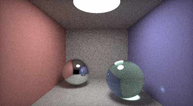
Since 4D space is more expansive, point light sources decay by inverse cube law, and light reflection is more chaotic, so there’s more noise at the same sampling rate. You need to click the play button and wait longer to see clear image quality. You should see that the 3D and 4D scenes look completely identical from the initial angle (except for slight light differences). In the 4D scene, dragging up and down reveals these spheres changing size, possibly disappearing or new spheres appearing - these are all hyperspheres in 4D space. Another detail showing light propagation in 4D space: by dragging the cross-section to the right angle, you can discover another hypersphere not yet intersected by the screen cross-section through the reflection in the left mirror sphere.

You might think there’s still quite a bit to change from 3D to 4D, but actually if you don’t use random reflection sampling and instead use lighting models that stop at diffuse reflection, you really only need to change vec3 to vec4. Finally, since RTX and similar ray tracing acceleration cards are specifically designed for triangle intersections in 3D space, they can’t accelerate tetrahedron intersections. Since I haven’t really worked with ray tracing pipelines, I can’t rule out the possibility of “disguising” 4D data as 3D data for processing (though I suspect feasibility is low).

1.2 Rasterization Methods

Now let’s discuss the more common rasterization rendering methods. The basic primitives GPUs can handle - points, lines, triangles - are all mathematical simplices. We naturally think 4D scenes need to rasterize tetrahedra. But since GPUs don’t have hardware optimized for voxelizing tetrahedra, we can only write general parallel computing programs to implement this. The tetrahedron rasterizer I tested using compute shaders (a type of GPU program that processes arbitrary data rather than rendering graphics) wasn’t very efficient (see this example in tesserxel). Unless you specifically develop a tetrahedron rasterization chip, to maximize existing hardware performance advantages, layered rendering is generally adopted - computing and rendering cross-sections of 3D images rather than rendering one tetrahedron at a time. So we’ll focus on slice rasterization methods.

Without considering complex optical phenomena, just from the two steps of finding graphic cross-sections and projections, their order is interchangeable. That is, the 2D cross-section of a 3D image captured by a camera of a 4D scene has the same geometric data as a 3D cross-section of a 4D scene then captured as a 2D image. Now, how to quickly calculate cross-sections of 4D objects becomes the top problem in 4D computer graphics. There are various methods for calculating cross-sections. I’ll introduce all the methods I know.

Tetrahedron Method

Intersecting a tetrahedron with a plane may yield a triangle or quadrilateral. We can substitute the four vertices of the tetrahedron into one side of the plane equation and determine by sign whether they’re on the same side. If all 4 points are on one side, there’s no intersection. If the two sides have 1 and 3 points respectively, we get a triangle. If each side has two points, we get a quadrilateral.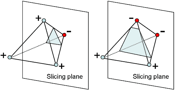

How to implement this programmatically? GPUs don’t have functionality for handling tetrahedron cross-sections, so the simplest brute force method is to have the CPU pre-calculate cross-sections of the 4D scene before each render, obtaining a 3D scene, then send it to the GPU for rendering using traditional 3D rendering techniques. However, its disadvantage is that CPU cross-section calculation becomes very heavy for complex scenes. We want to calculate tetrahedron cross-sections in parallel on the GPU for significantly improved efficiency. Since GPU workflows (rendering pipelines) are designed for common 3D rendering without cross-section calculation functionality, we need various tricks to implement this. Below I’ll introduce three methods based on the type of shader used for cross-section calculation.

1. Vertex Shader Cross-section Calculation
   This is the algorithm used by YouTuber CodeParade in the game 4D Golf. Each tetrahedron has four vertices. Finding the cross-section may yield an empty set, triangle, or quadrilateral, so the GPU may ultimately draw 0-2 triangles, outputting at most four vertices. We can package all four vertex data of each tetrahedron and duplicate it four times, adding numbering from 0 to 3 as vertex input. This allows the GPU to run four times in the vertex shader to calculate the final coordinates of the four vertices of the cross-section. Note that since we need to determine vertex numbering and whether vertices are on the same or different sides of the plane to determine the final cross-section, the shader will be filled with many conditional branch statements that affect parallel computing efficiency. CodeParade uses a pre-calculated texture map to avoid them through table lookup, detailed in this YouTube video.

2. Geometry Shader Cross-section Calculation
   This paper developed a 4D graphics rendering library called gl4d using another approach: In most GPU rendering pipelines, an optional geometry shader can be inserted between the vertex shader and rasterizer. This geometry shader can accept vertex shader input and output any number of basic primitives under programmer control. Directly controlling quadrilateral cross-section output makes this shader seem specifically designed for calculating cross-sections! Since the geometry shader comes after the vertex shader, it accepts all vertices of primitives transformed by the vertex shader, so we need to combine four vertex coordinates into one primitive. Known basic primitives only include points, lines, and triangles, none with 4 vertices. Fortunately, geometry shader designers anticipated these special needs and provided special primitives (Adjacency Primitives) that can only be used as geometry shader input. Using the gl_lines_adjacency primitive can pack exactly four vertices for the geometry shader to calculate, outputting 0 to 2 triangle primitives based on results (corresponding to no intersection, triangle cross-section, and quadrilateral cross-section). The geometry shader stage can also do back-face culling by vertex order. Compared to CodeParade’s method, this doesn’t require duplicating each tetrahedron’s data four times, but the disadvantage is some mobile GPUs may not have geometry shaders, or have them but with low execution efficiency.

3. Compute Shader Cross-section Calculation
   Since some devices don’t support geometry shaders, traditional web GPU programming interfaces WebGL and the latest WebGPU simply don’t include geometry shader functionality. But WebGPU provides a new “Compute Shader”. Compute shaders are designed for general parallel computing tasks beyond image rendering, such as big data machine learning scenarios. We can send tetrahedron vertex data to the compute shader, calculate cross-sections to get cross-section vertex data, then pass this data to the vertex shader in the traditional rendering pipeline to complete subsequent rendering work. Tesserxel uses compute shaders by default to handle 4D object cross-sections. Compute shaders process each tetrahedron in parallel, yielding 0 to 2 triangles. I use a large array to store these triangles. Since we can’t know the execution order of different parallel computing units (don’t know who’s fast or slow), when parallel program units write triangles to the large array, there may be “Data Race” - two parallel tetrahedron cross-section programs may simultaneously write triangle data to the same array cell, with later writes overwriting earlier ones. WebGPU provides “atomic” operations to avoid data races: we use an “atomic integer” type variable to store the array’s next free position index. When the first execution needs to read/write this atomic type variable, it “locks” it until it finishes reading the data value and updates the variable to the next free position index (simply incrementing the index value by one) before “unlocking”. If other programs execute to need reading/writing the locked atomic type variable, they stop there, waiting for the variable to unlock before executing. Since reading the variable and incrementing by one takes very little time, other programs don’t waste much time waiting to unlock, maintaining high parallelism.

Cell Complex Method

Cell Complex (CW-Complex) is a completely upgraded version of the tetrahedron method. Imagine using the tetrahedron method to draw a voxel cube - you first need to tetrahedralize the cube, getting at least 5 tetrahedra.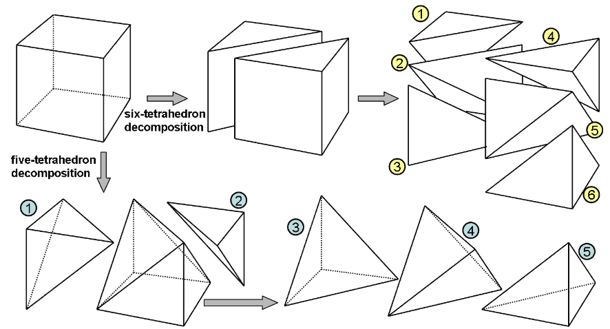If we want to subdivide complex shapes like a regular dodecahedron, there would be nearly thirty tetrahedra, but the dodecahedron’s cross-section is at most a decagon. This shows that compared to using all tetrahedra, directly handling polyhedra and polygons will reduce many unnecessary primitives. Cell complexes are generalizations of polyhedra, providing a method to describe 4D objects without using tetrahedra. Cell complexes record four types of data: vertices, edges, faces, and cells. Vertex data is coordinate vector arrays, edge data is the indices of its two endpoints in the vertex array, each face in face data records the indices of all edges composing it in the edge array, and cell data is the indices of faces surrounding it in the face array. Things constructed layer by layer this way are called cell complexes, generalizable to arbitrary dimensions.

Taking the above cube cell as an example, its data structure is like this: (array indices written as subscripts, corresponding to the figure above)

Vertices: {(1,1,1)₀,(1,1,-1)₁,(1,-1,1)₂,(1,-1,-1)₃,(-1,1,1)₄,(-1,1,-1)₅,(-1,-1,1)₆,(-1,-1,-1)₇}
Edges: {(0,1)₀,(1,3)₁,(2,3)₂,(0,2)₃, (4,5)₄,(5,7)₅,(6,7)₆,(4,6)₇, (0,4)₈,(1,5)₉,(2,6)₁₀,(3,7)₁₁}
Faces: {(0,4,8,9)₀,(1,5,9,11)₁,(2,6,10,11)₂,(3,7,8,10)₃,(0,1,2,3)₄,(4,5,6,7)₅}
Cells: {(0,1,2,3,4,5)₀}

Although the cell complex data structure is intuitive, how do we find cross-sections of such complex hierarchical things? As long as the shape is convex, we can actually use a layered algorithm to accomplish this task:

1. First calculate whether all vertices are on different sides of the hyperplane;
2. For each edge, check if its endpoints cross the plane; if so, calculate intersection coordinates;
3. For each face, check if its edges produced intersections in the previous step; if so, construct the cross-section shape’s edges from these intersections. (Note: if the shape isn’t required to be convex, there may be more than two intersections, yielding “illegal” edges with more than two endpoints, and the algorithm can’t continue)
4. For each cell, check if its faces produced intersection lines in the previous step; if so, construct the cross-section shape’s faces from these lines.

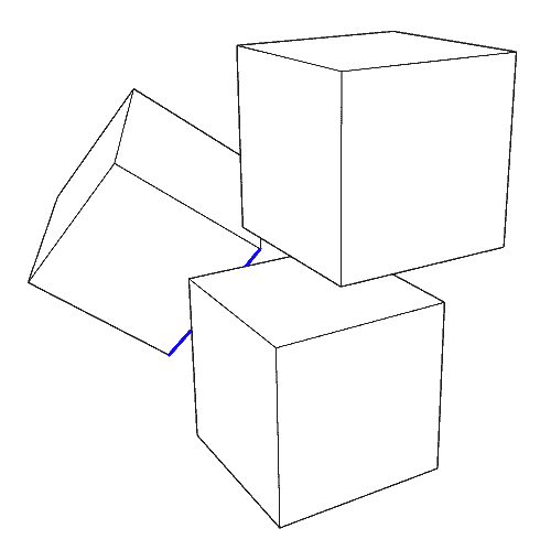
Taking the blue cross-section in the cube below as an example, we additionally record such a structure. Note if all boundaries of a cell aren’t intersected, that cell is ignored, shown in gray in the figure:

Vertices: {+₀,-₁,-₂,-₃,+₄,+₅,+₆,-₇}
Edges (new vertices): {(+0,-1)₀,(-1,-3)₁,(-2,-3)₂,(+0,-2)₃, (+4,+5)₄,(+5,-7)₅,(+6,-7)₆,(+4,+6)₇, (+0,+4)₈,(-1,+5)₉,(-2,+6)₁₀,(-3,-7)₁₁}
Faces (new edges): {(0,4,8,9)₀,(1,5,9,11)₁,(2,6,10,11)₂,(3,7,8,10)₃,(0,1,2,3)₄,(4,5,6,7)₅}
Cells (new faces): {(0,1,2,3,4,5)₀}

Finally, to render the newly constructed cross-section cell complex, non-triangular faces still need triangulation, but triangulating after taking cross-sections produces far fewer primitives than tetrahedralizing from the start. How to triangulate? Since we assumed the shape is convex, we can simply select a vertex and connect lines to all non-adjacent vertices.

Although cell complexes have much less total computation than tetrahedra, currently they only seem suitable for CPU execution, because this algorithm must execute sequentially from vertices to edges to faces, and even at the same parallelizable level, each face and cell generally has different numbers of boundaries, making parallel efficiency difficult even with parallelization. My old 4dViewer (except Minecraft4d) used CPU-calculated cell complex cross-sections to render 4D scenes. With not too many object faces, the speed is actually acceptable, even rendering hyperspheres without pressure.

Cell complexes have another disadvantage - difficulty representing texture coordinates (4D objects in 4dViewer except Minecraft4d all have pure color surfaces, no textures…) Unlike storing texture coordinates directly on each tetrahedron’s four vertices then getting each interior point’s coordinates through linear interpolation, cell complex data structures only directly contain information about faces surrounding cells, without explicitly included vertex information. If a cell’s tetrahedron subdivision (or its cross-section’s triangulation) differs, texture coordinates obtained by interpolating middle points will also differ. Therefore, my current Tesserxel engine doesn’t directly use cell complexes to represent 4D objects to be rendered, only as a 4D modeling tool - cell complex models must be converted to tetrahedra before rendering. I plan to expand on this in the next article about 4D graphics modeling.

Output Cross-section Vertex Coordinates

After finding cross-sections, the next step is rendering. Regardless of which method above, we encounter the same two problems - view frustum culling and occlusion culling. By analogy with 3D space, rendering 4D geometry requires a 5D homogeneous vector: its first three components are positions on the voxel canvas, the fourth is depth buffer for handling front-back occlusion relationships, and the last is for perspective division. All GPUs in the world are currently designed for 3D rendering, without 5th order matrices and 5D vec5 vectors, and the rasterizer hardware level lacks corresponding processing logic. Fortunately, we’re only drawing one cross-section of a 4D object at a time, so we can do this:

1. First perform coordinate transformation on tetrahedron vertices to get 5D homogeneous coordinates. Since vec5 data type isn’t provided, we can use a float variable and a vec4 variable to store them separately.
2. Calculate cross-section data in homogeneous coordinates (calculation methods can be simply derived from ordinary coordinate systems), finding intersection homogeneous coordinates.
3. Assume the cross-section is perpendicular to some coordinate axis of the voxel image. Since intersections must lie within the cross-section, we can directly ignore the now-useless coordinate perpendicular to the cross-section, reducing the homogeneous vector dimension to four, sending it as the final vertex shader output to the GPU to handle view frustum culling and occlusion culling as ordinary 3D graphics.

For cell complexes calculated on the CPU side, there’s another method to reduce CPU computation: Logically we need to transform model vertex coordinates to camera coordinates then calculate cross-sections. These operations are slow when all done in CPU. We can actually optimize by first transforming the cross-section equation to model coordinates in CPU to directly calculate cross-sections, then send to GPU to transform all vertices to camera coordinates.

Rasterization Method Process Summary

I use a diagram to summarize these method processes:

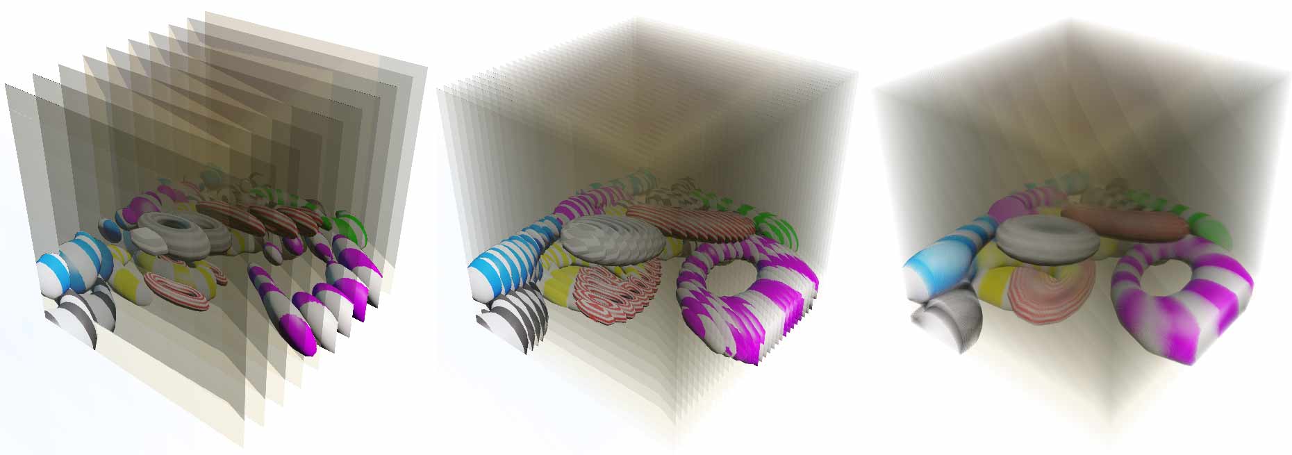
Finally finished writing about 4D object cross-section rasterization rendering methods, but these single cross-sections aren’t yet voxel photos. How to render voxels? First we render single cross-section images to a texture for storage using Frame Buffer technology, then we can use GPU-provided Alpha Blending technology to paste these single-layer photo textures onto translucent layers and stack them up. When there are enough layers, it looks like a voxel cloud. Generally we render one layer then immediately project it onto the 2D canvas for alpha blending, so drawing the next layer can reuse the frame buffer texture just used, saving video memory. To stack up nice-looking voxel clouds, we can work from three aspects:

1. Give different objects in the scene different opacities, like ground and sky can be more transparent, objects can be more opaque. This greatly increases the visibility of small objects needing attention in voxel clouds, like the almost opaque “donut” in the image below;
2. Dynamically change voxel slice division direction based on the direction projecting voxels to 2D screen. Generally layering by coordinate axes is sufficient. If layering by arbitrary directions, the overhead introduced by calculating layer cross-section shapes and positions isn’t worthwhile;
3. Can adjust opacity pixel by pixel in fragment shader through exponential decay laws of light propagation in uniform media, i.e., the proportion of light passing through each cross-section layer. When facing the cross-section directly, light travels a short distance between two cross-section layers, so decay should be small and more transparent. When viewing angle to cross-section is large, distance between two cross-section layers is long, so decay should be large and more opaque.
   

Supplement: Glasses-free 3D Rendering Technology

Both 4DBlock and my Tesserxel support glasses-free 3D, displaying left and right images with slight differences to give pictures stereoscopic depth. As previously detailed in “The 4D World (5): Experiencing 4D Vision and Sense of Direction”, the depth sense direction of 3D stereoscopic photos is the stereoscopic photo’s depth, while the depth sense direction needed for cross-section images is the true front-back direction of the fourth dimension’s distance from camera. These two types of glasses-free 3D are implemented differently.

1. 3D stereoscopic photo depth sense: To obtain 3D stereoscopic photo depth sense, we need left and right cameras each offset by a certain horizontal distance. Since voxel photos are given, when rendering each cross-section projection onto canvas, we only need to draw the layered slices to be textured twice at different angles without re-rendering cross-sections. The additional drawing overhead can be said to be very small. (But actually Alpha blending overhead isn’t small, this can’t be avoided…)
2. Single cross-section view depth sense: Since this is fourth-dimensional front-back depth, we need to set up two closely spaced cameras in the 4D scene. Does this mean we need to render all objects twice at two positions? Actually, although camera positions are offset, this offset is still within the same hyperplane cross-section (otherwise left and right eyes would see completely different things, unable to produce stereoscopic sense), so the intersected geometric data is the same. Therefore we can just give different offsets when finally outputting vertices. That is, first doing cross-section then offset within cross-section is equivalent to first doing offset within cross-section then doing cross-section. But this requires that cross-section calculation and final vertex output shader are two steps in the GPU’s 4D cross-section rendering pipeline. Otherwise if these two steps can’t be separated, there’s no room for this optimization. For example, CodeParade’s single vertex shader completes everything and has no room for this optimization. Also note that if back-face culling was done in the cross-section calculation stage, it’s not suitable for this optimization, because after camera angle deviation, some faces may face one eye while backing the other.

That’s it for voxel/cross-section rendering. Now let’s look at something completely different - non-voxel/cross-section rendering.

2. Stereographic Projection Method

Visualizing 4D graphics doesn’t necessarily require calculating “real” light ray color information. For example, the well-known stereographic projection essentially projects graphics on a hypersphere - a curved 3D space - onto 3D space. It’s essentially a mapping between 3D spaces, strictly speaking not involving 4D, so it’s almost impossible to use for displaying complex “real” 4D scenes, generally only used for displaying 4D convex geometric objects.

Rasterization Triangle-based Method

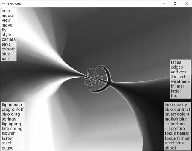
With a bit of analytic geometry, it’s easy to derive stereographic projection transformation formulas. The simplest method is to project 4D vertex coordinates on the hypersphere to 3D, nothing special. For example, the stereographic projection software Jenn3D. Two things to note:

1. Since original models must have coordinates on the hypersphere, creating edges and vertices with certain thickness requires developers to be very familiar with spherical geometry.
2. Since distortion increases closer to the north pole, it’s recommended to dynamically increase polygon mesh subdivision near the north pole, otherwise you’ll get the situation below.

Ray Tracing-based Method

Stereographic projections from triangle methods become non-smooth due to mesh precision issues, while high-precision ray tracing can avoid this problem. For specific principles, see this interactive webpage and this Shadertoy example (click the image below to activate rendering, drag mouse left-right to select different regular polytopes):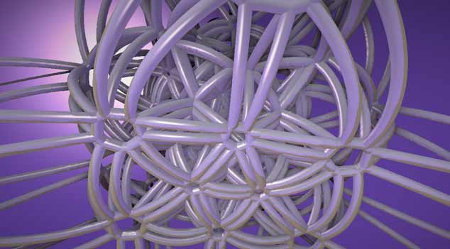

3. Wireframe Rendering

Since we humans naturally don’t have 3D retinal eyes that can simultaneously see all voxels inside 3D, voxel rendering brings lots of color overlap. Wireframe rendering can greatly reduce overlapping pixels, lowering comprehension difficulty (though this is only reduced in some aspects - there are always tradeoffs). So in the 4D computer graphics field, wireframe rendering is actually used more than voxel color rendering. For example, 4DBlock, dearsip and yugu233 all use this method to visualize 4D objects.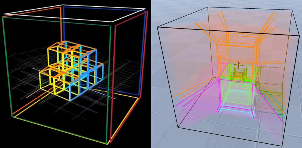

There’s not much to say about simply rendering wireframes: first transform vertices to coordinates on the 3D camera’s photosensitive hyperplane, getting coordinates similar to those in voxel images, then project 3D coordinates to 2D, then connect endpoints to draw line segments. But this algorithm has two big problems - still those two problems - view frustum culling and occlusion culling.

View Frustum Culling

Since line segments to be drawn can completely have one end in front of the camera and one behind, directly doing perspective division in perspective projection will cause chaotic results. Also, since we’re no longer using rasterization methods for drawing, this requires us to manually calculate intersections of line segments with the view frustum, keeping only intersecting parts. Actually not just front and back, now we must also manually clip top, bottom, left, right, front and back sides.

The More Troublesome Problem - Occlusion Culling

Since we’re now drawing lines directly on the final 2D screen without layered rendering, we can’t get depth buffer for occlusion culling. So we must analytically calculate coordinates where occlusion relationships between line segments and each face change, like ray tracing. How to do this? Treat the camera as a light, the shadow area behind each face (cell) is the area it occludes. Our task is to calculate the intersection of line segments with this area and cull them. These areas are all bounded by hyperplanes, solving intersections isn’t complex. The hard part is determining occlusion relationships. Here I’ll introduce the algorithm in Block4d.

For each $n-1$ dimensional cell of an $n$-dimensional convex polytope, first determine by normal whether it’s front-facing or back-facing from the camera’s view. Then for each $n-2$ dimensional ridge of the convex polytope, see if it’s at a viewing angle corner, i.e., whether the cells on both sides have one judged as front-facing and the other as back-facing. Then we record the hyperplane containing the camera and corner ridge, along with recording hyperplanes of all cells facing the camera front-on. We get an infinitely large conical occlusion region - any line segment within this region will be clipped.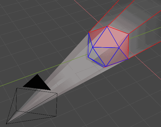The specific clipping idea is simple: the occlusion region is bounded by hyperplanes, only points inside all hyperplanes are interior points. In other words, for a given point, as long as we detect it’s outside some hyperplane, it definitely won’t be clipped. The specific algorithm is as follows:

First prepare an array $P$ storing hyperplanes bounding the conical clipping region, with normals already adjusted to uniformly point outward. Then set the first endpoint A’s position as 0, second endpoint B’s position as 1. We prepare two temporary variables $a$ and $b$ to store clipping positions on the line segment, with the region between them considered the occlusion region:
Left endpoint A(0)——a—–occlusion region—–b——(1)Right endpoint B
Initialize $a=0$ and $b=1$, representing the line segment is completely occluded:
Left endpoint A(0=a)———occlusion region——–(b=1)Right endpoint B
Below we enter a loop, checking the line segment’s two endpoints for each hyperplane, gradually finding safe (i.e., not occluded) intervals, slowly compressing the clipped range:

For each hyperplane p in the conical clipping region's hyperplane array P:
  Calculate which side of plane p endpoints A, B are on;
  If endpoints A, B are both outside plane p:
    Directly determine entire line segment is not occluded, algorithm ends;
  If endpoint A is outside plane, endpoint B inside plane p:
    Calculate intersection position x of line segment with plane;
    If x>a then update a to x; (Expand the safe interval confirmed not to be occluded)
  If endpoint B is outside plane, endpoint A inside plane p:
    Calculate intersection position x of line segment with plane;
    If x<b then update b to x; (Expand the safe interval confirmed not to be occluded)

Note the above code seems to have three cases in the loop, but there’s an implicit fourth: if both endpoints are completely inside the hyperplane, there’s no valid information. In this case nothing needs to be done, just continue the loop, so it’s not written out.

It seems we’ve perfectly solved the problem, but there’s actually another case: when the camera enters inside the polytope, if we want to implement culling like in the image below, the above algorithm no longer applies (at this time hyperplane array P is empty). The culled part now reverses to become the exterior, and the algorithm adjusts accordingly: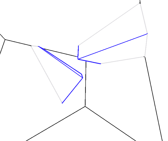

Still prepare two temporary variables $a$ and $b$ to store clipping positions on the line segment, but now the middle region becomes the safe unoccluded region:
Left endpoint A(0)—–occlusion region—–a——–b—–occlusion region—–(1)Right endpoint B
Still initialize $a=0$ and $b=1$, but now it represents the line segment is completely unoccluded:
Left endpoint A(0=a)——————(b=1)Right endpoint B
Below we enter a loop, checking the line segment’s two endpoints for each hyperplane, gradually finding regions to cull, slowly compressing the safe range:

For each hyperplane p in the conical clipping region's hyperplane array P:
  Calculate which side of plane p endpoints A, B are on;
  If endpoints A, B are both outside plane p:
    Directly determine entire line is completely occluded, algorithm ends;
  If endpoint A is outside plane, endpoint B inside plane p:
    Calculate intersection position x of line segment with plane;
    If x<b then update b to x; (Expand culling region)
  If endpoint B is outside plane, endpoint A inside plane p:
    Calculate intersection position x of line segment with plane;
    If x>a then update a to x; (Expand culling region)

For scenes with multiple objects, we need to continue culling on line segments remaining after previous culling. Note when the camera is outside, the case $0 < a < b < 1$ corresponds to the line segment being split in two with the middle part culled (refer to the blue line segment in the first image of the occlusion culling section). It’s treated as two line segments participating in the next round of occlusion culling by other cells. Finally, there’s a small detail: to avoid floating point errors when drawing polytope surface ridges, the polytope’s faces to be culled can be shrunk inward by a very small value.

That’s the culling process for line segments with one convex polytope. However, the complex culling logic of wireframe rendering makes it well-implemented on CPU but difficult to port to GPU. I haven’t found parallelized algorithms yet, though some limited optimization can still be done with hierarchical data structures (like bounding boxes). Worth mentioning, dearsip also implemented 3D cell occlusion culling of 2D faces. Most objects in his scenes are axis-aligned hypercubes. Under this constraint, 2D face occlusion culling is relatively easy, but culling arbitrary-shaped 2D faces is actually very complex. I haven’t studied his source code yet, don’t know how he implemented it. I’ll supplement when I figure it out. If readers know other 4D visualization methods and are interested in their rendering principles, welcome to discuss.