2016-04-23

Four-Dimensional Space (VII): N-Dimensional Vectors

Image from en.wikipedia: Geometric meaning of multivectors

# This series discusses geometry in pure space, but some properties of k-vectors discussed in this article also hold in four-dimensional spacetime (just with different metrics). This article requires high mathematical ability: many mathematical formulas will appear. k-vectors have applications in physics beyond relativity (spacetime), see CFY’s article Angular Velocity, Axial Vectors, 2-Vectors which introduces k-vectors from another angle—physics.

Featured Content

Using “2-dimensional vectors” to represent planes
Calculating angles using vector inner and outer products
Singular (compound) 2-vectors
2-vectors analyzing rotation

　　It’s time to discuss quantitative calculations in four-dimensional space. On one hand, this can verify the correctness of our geometric intuition, otherwise our intuition is just blind guessing without evidence; on the other hand, calculations are essential for programming four-dimensional graphics.

Vectors No Longer Suit Four-Dimensional Geometry

　　Everyone should know about n-dimensional vector dot and cross products for calculating angles and normal vectors. The dot product has long been extended to N dimensions, so calculating line-line angles is no problem. In three-dimensional space, when we encounter a plane, we use its normal vector to participate in angle calculations—because the plane’s normal vector direction is unique; for three-dimensional cells in four-dimensional space, we also use their normal vectors for calculations—because their normal vector direction is also unique. But the problem is: a plane’s normal vector is not unique—because in four-dimensional space, a plane’s normal space is also two-dimensional, meaning the normal plane is also a plane. This way we can never convert to vector solutions!
　　Of course, planes can be written in analytical form: the intersection of two cell equations, but it’s too cumbersome—do you like using intersection equations to represent lines in solid geometry?
　　Planes can be represented by vectors: $\vec x=\lambda\vec m+\mu\vec n {,}\lambda,\mu\in \mathbf R$, but the choice of vectors and parameters here is arbitrary, and it’s inconvenient for calculations. We can only break through on another level: extend the cross product to higher dimensions.

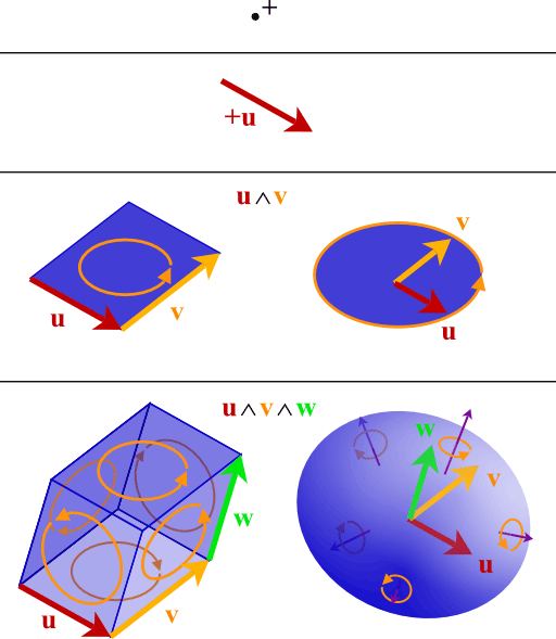
　　Of course, we have another path: directly use a vector-like quantity to represent planes, which can do inner and outer products with other vectors, thus conveniently calculating projections and angles. This new quantity is called a 2-vector (bivector). From our previous analysis, 2-vectors represent planes, and planes are spanned by two non-collinear ordinary vectors (1-vectors), so we define an operation “$\vec a\wedge\vec b$” between two 1-vectors, which we call the wedge product.
　　Since we wanted to generalize the outer product (cross product), we bring it over and combine the two: $\vec a\wedge\vec b$ is a quantity with magnitude and directional orientation: the orientation is the plane spanned by $\vec a$ and $\vec b$, following the right-hand rule (meaning $\vec a\wedge\vec b=-\vec b\wedge\vec a$), and the magnitude (norm) is the area of the parallelogram spanned by $\vec a$ and $\vec b$, so if $\vec a$ and $\vec b$ are collinear, then $\vec a\wedge\vec b=0$. This idea is good, but it’s not useful yet, because we still need to see how to represent and calculate it in coordinates.

Wedge Product and 2-Vectors

Three-dimensional case
　　This is a mathematical tool we haven’t used even in three-dimensional space. So let’s first discuss and familiarize ourselves with it in three-dimensional space, then generalize to four and N dimensions. Let $\vec m=(x_1,y_1,z_1), \vec n=(x_2,y_2,z_2)$, then

$\vec m\wedge\vec n=(x_1\vec e_x+y_1\vec e_y+z_1\vec e_z)$ $\wedge(x_2\vec e_x+y_2\vec e_y+z_2\vec e_z)$.
　　How to expand the parentheses? If $\wedge$ satisfies distributivity, the parentheses can be expanded! Let’s first assume it does, expand, and use $\vec a\wedge\vec b=-\vec b\wedge\vec a$ to simplify and combine (we also need to assume it’s a linear operator to combine): $\vec m\wedge\vec n=(x_1y_2-x_2y_1)e_x\wedge e_y + (x_1z_2-x_2z_1)e_x\wedge e_z + (y_1z_2-z_2y_1)e_y\wedge e_z$

　　Look familiar? This is the cross product formula we know. We transferred the cross product to the “$\wedge$” operation, so deriving the cross product formula is normal. This 2-vector has three independent components $e_x\wedge e_y$, $e_y\wedge e_z$, $e_x\wedge e_z$, which represent unit $xy$, $yz$, $xz$ planes, corresponding exactly to normal vectors $\vec e_z$, $\vec e_x$, $-\vec e_y$ (note this correspondence follows the right-hand rule, sometimes differing by a sign), giving the impression they are isomorphic (identical). But $\vec a\wedge\vec b$ and $\vec a \times \vec b$ have essential differences: the former represents a plane, the latter represents the plane’s normal line. We just found a special correspondence between them:

$a(e_x\wedge e_y)+b(e_y\wedge e_z)+c(e_x\wedge e_z)\to a\vec e_z+b\vec e_x+c\vec e_y$

This correspondence is called the Hodge dual, which we’ll use extensively later.

Four-dimensional case
　　In four-dimensional space, lines and planes (2-vectors) no longer have a one-to-one correspondence:
　　Let $\vec m=(x_1,y_1,z_1,w_1), \vec n=(x_2,y_2,z_2,w_2)$, then$$\begin{align} \vec m\wedge\vec n&=(x_1\vec e_x+y_1\vec e_y+z_1\vec e_z+w_1\vec e_w)\wedge(x_2\vec e_x+y_2\vec e_y+z_2\vec e_z+w_2\vec e_w) \\ &=(x_1y_2-x_2y_1)e_x\wedge e_y+(x_1z_2-x_2z_1)e_x\wedge e_z+(x_1w_2-x_2w_1)e_x\wedge e_w+(y_1z_2-z_1y_2)e_y\wedge e_z+(y_1w_2-w_1y_2)e_y\wedge e_w+(z_1w_2-w_1z_2)e_z\wedge e_w\end{align}$$
　　We see that 2-vectors in four-dimensional space have six independent components, which are pairwise combinations of coordinates, with component magnitudes being cross multiplication then subtraction of the two coordinates. Good, we can finally represent planes.
Return to Contents

2-Vector Inner Product and Its Meaning

　　The next step is to define the inner product between 2-vectors: the most natural definition is to multiply corresponding components and add them, i.e.$$\begin{align} A&=a_1e_{xy}+b_1e_{xz}+c_1e_{xw}+d_1e_{yz}+e_1e_{yw}+f_1e_{zw} \\ B&=a_2e_{xy}+b_2e_{xz}+c_2e_{xw}+d_2e_{yz}+e_2e_{yw}+f_2e_{zw} \\ then A\cdot B&=a_1a_2+b_1b_2+c_1c_2+d_1d_2+e_1e_2+f_1f_2 \end{align}$$
($e_{ij}$ is shorthand for $e_i\wedge e_j$, same below)
　　Let’s write the angle formula:
$$\lvert cos\langle A,B\rangle\rvert={\lvert A\cdot B\rvert\over \lVert A \rVert \lVert B \rVert}$$
　　Here the norm (magnitude) of a 2-vector is of course the square root of the 2-vector’s inner product with itself. It seems all problems are solved! But wait, something’s not right: only one angle appears here! We analyzed earlier that two angles are needed to represent the relationship between planes.
　　For example, let’s do some simple calculations:
The angles between $e_{xy}$ and $e_{xy}$, $e_{xy}$ and $e_{xz}$, $e_{xy}$ and $e_{zw}$ are: 0°, 90°, 90° respectively.
Well, the angle cosine of the $xy$ plane with itself is certainly 0°, but the latter two are both 90°: does this angle we calculated have meaning? What’s its relationship with the two angles that measure planes?
　　Remember the generalization of the projection area theorem from the last article? We boldly conjecture: the essence of the 2-vector inner product is one area quantity multiplied by another area quantity’s projection onto it, so we get the geometric meaning of the dot product between area quantities in four-dimensional space:
$$\lvert cos\langle A,B\rangle_1cos\langle A,B\rangle_2\rvert=\lvert cos\theta_1cos\theta_2\rvert={\lvert A\cdot B\rvert\over \lVert A \rVert \lVert B \rVert}$$
This formula has the same function as the projection area theorem. Generally, one equation with two unknowns cannot solve for $\theta_1, \theta_2$. No problem, at least we’ve obtained a coordinate solution method, while the projection area theorem is a geometric method.
The 2-vector inner product is very similar to the vector inner product, so we can also deduce: only when two bivectors have proportional corresponding components ($A=kB, k\in \mathbf R$) do we have $\lvert cos\theta_1cos\theta_2\rvert=1$, i.e., $\theta_1=\theta_2=0$. So just like vectors, if two 2-vectors are proportionally “collinear”, they represent the same plane. Actually, the converse is also true, which we won’t prove here.

Generalizing the Cross Product

Hodge Dual

　　Recall the relationship between $\vec a \times \vec b$ and $\vec a\wedge\vec b$: they are mutually perpendicular, orthogonal complements, with the same magnitude (norm) and components, but different geometric dimensions and meanings. We define the Hodge dual mapping: mapping a k-vector to its orthogonal complement $(N-k)$-vector. We denote the Hodge dual of $A$ as $*A$, where N is the space dimension, and we’re discussing the case N=4. The Hodge dual also requires that the $(N-k)$-vector has the same magnitude (norm) as the k-vector, and the direction of the $(N-k)$-vector follows the right-hand rule—we can’t gesture with our right hand in high dimensions, but this is actually an abstract rule. Let’s illustrate with specific examples:
$*e_{xy}=e_{zw}$, $*e_{yz}=e_{wx}$, $*e_{zw}=e_{xy}$, $*e_{wx}=e_{yz}$
As long as we ensure the subscripts cycle from left to right as xyzw yzwx zwxy wxyz, the equations hold. Otherwise, arbitrarily swapping the positions of two letters in the order will change the sign. For example, $*e_{xy}=e_{zw}$, but $*e_{xz}=-e_{yw}$. In mathematics, this is called odd and even permutations. (Similar to the alternating signs in determinants)
$$\begin{align}Let F&=a_1e_{xy}+b_1e_{xz}+c_1e_{xw}+d_1e_{yz}+e_1e_{yw}+f_1e_{zw} \\ then *F&=f_1e_{xy}-e_1e_{xz}+d_1e_{xw}+c_1e_{yz}-b_1e_{yw}+a_1e_{zw} \end{align}$$

2-Vector Outer Product

　　Now we can describe the essence of the cross product: an m-vector and n-vector cross product in N-dimensional space yields an (N-m-n)-vector: it’s the orthogonal complement of the space spanned by the m-vector and n-vector (an (m+n)-vector), with direction following the right-hand rule. (Note: this is just one generalization of the vector cross product, used only in this subsection. Later we’ll use the $\times$ symbol to denote another operation between 2-vectors similar to the vector cross product called the mixed product)
For example, 2-vectors $F\times G=*(F\wedge G)$. Note here $F\wedge G$ is a 4-vector! This time we also need to assume the operation $\wedge$ is associative, i.e., $(A\wedge B)\wedge C=A\wedge (B\wedge C)$.
　　$$\begin{align} Let F&=a_1e_{xy}+b_1e_{xz}+c_1e_{xw}+d_1e_{yz}+e_1e_{yw}+f_1e_{zw} \\ G&=a_2e_{xy}+b_2e_{xz}+c_2e_{xw}+d_2e_{yz}+e_2e_{yw}+f_2e_{zw} \\ Combining &and simplifying: \\ F\times G&= (a_1f_2-b_1e_2+c_1d_2+d_1c_2-e_1b_2+f_1a_2)e_{xyzw}\end{align}$$
The Hodge dual of $e_{xyzw}$ is a 0-vector, i.e., “scalar”: “1”. This “scalar” is not a true scalar, because it changes sign under spatial reflection transformations (the right-hand rule at work), so we call it a pseudo-scalar.
Note: we haven’t defined $F\wedge G=-G\wedge F$, $F\wedge F=0$ for 2-vectors. Actually $F\times G=G\times F$ because when we swap variables, the subscripts change from 1234 to 3412, with an even number of swaps, so the negative signs cancel! So we can happily use commutativity again. Similarly, $**F=F$, but this conclusion doesn’t necessarily hold for other k-vectors.
Finally, we obtain: the cross product between 2-vectors also yields a scalar. We notice its form is very similar to the inner product of two vectors—both are sums of multiplication terms. In fact, we have: $F\times G=F\cdot (*G)=G\times F=G\cdot (*F)$.

Geometric Meaning

$A \times B$ is a scalar: its absolute value equals the hypervolume of the parallelepiped they span (think of a parallelepiped): how do two planes span a parallelepiped? If $A=\vec a\wedge \vec b$, $B=\vec c\wedge \vec d$, then $A\wedge B=\vec a\wedge \vec b\wedge \vec c\wedge \vec d$—actually the parallelepiped formed by these four vectors. This definition is well-defined, because if $\vec a_1\wedge\vec b_1=\vec a_2\wedge\vec b_2=A$, although the parallelepipeds enclosed by $\vec a_1, \vec b_1, \vec c, \vec d$ and $\vec a_2, \vec b_2, \vec c, \vec d$ have different shapes, it can be proven that their volumes are the same.

For convenience, let’s first choose a special pair $\vec a\wedge \vec b=A$: where $\vec a, \vec b$ are vectors parallel to the directions of maximum and minimum angles between the two planes (their angles with $B$ are $\theta_1, \theta_2$). The four-dimensional volume of the parallelepiped $V_4=V_3h$. $V_3$ refers to the three-dimensional volume of any parallelepiped cell in the parallelepiped (like the green one in the figure), $h$ is the height corresponding to this cell in the parallelepiped. And $V_3=SH$. From geometric relationships: $h=\lVert\vec a\rVert sin\theta_1$, $H=\lVert\vec b\rVert sin\theta_2$, we get: $V_4=S\lVert\vec a\rVert\lVert\vec b\rVert sin\theta_1 sin\theta_2=\lVert A \rVert \lVert B \rVert sin\theta_1 sin\theta_2$
Return to Contents

Perfect Solution to the Problem!

$$\lvert \cos\theta_1\cos\theta_2\rvert={\lvert A\cdot B\rvert \over \lVert A \rVert \lVert B \rVert} $$$$ \lvert \sin\theta_1\sin\theta_2\rvert={\lvert A\times B\rvert\over \lVert A \rVert \lVert B \rVert}$$
　　Two equations, two unknowns, we can solve for the two angles! Can all angle problems in N-dimensional space be done this way? Unfortunately, this method only works in four and five dimensions—in six dimensions, two cells need three angle parameters for description, but inner and outer products only give two equations, so you’ll have to honestly use linear algebra.
　　Fortunately, we’re not concerned with higher dimensions for now. Back to four-dimensional problems: given a vector $\vec m$ and a 2-vector $A$, how do we calculate the angle between them (line-plane angle)? We hope the previous formulas continue to hold. But the inner product is multiplication of corresponding terms, and in four-dimensional space vectors have 4 components while 2-vectors have 6 components, so we can’t calculate the inner product. So we have to use the outer product—let’s calculate: $\vec m\wedge A$. After simplification, we get a 3-vector: $ ae_{xyz}+be_{yzw}+ce_{zwx}+de_{wxy}$, which maps through Hodge duality to the vector $ae_w+be_x+ce_y+de_z$. Obviously, its magnitude (norm) represents the volume of the parallelepiped formed by $m$ and $A$, and its direction is the normal to the cell containing this parallelepiped—just like the mixed product, its geometric meaning is clear:
$$\lvert sin\theta\rvert={\lVert\vec m\times A\rVert\over \lVert \vec m \rVert \lVert A \rVert}$$
Since the line-plane angle requires only one angle, we don’t need to use the inner product anymore. Now we seem to have powerful computational tools, but are these conclusions correct? You can verify by using the 2-vector method to find line-plane angles, plane-plane angles, etc. in hypercubes and comparing with results obtained by geometric methods. I’ve verified many cases, and the results from both methods are always the same.

Dark Clouds

Previously, geometry led algebra; now let’s try to think about some problems in reverse:

Four-dimensional space is not intuitive, these derived things have no rigorous proof, correctness cannot be guaranteed;
The concept of 2-vector “direction” is vague;
Vector addition has intuitive meaning: the diagonal of a parallelogram; does the plane corresponding to 2-vector addition have a geometric interpretation? What plane does $e_{xy}+e_{zw}$ represent? What about $e_{xy}+e_{xz}+e_{xw}$?

Let’s answer one by one:

First, proof is not a problem: we can first abstractly define a linear operator $\wedge$ satisfying certain properties, then show it has a one-to-one correspondence with planes, then use linear algebra to prove everything that follows.
When calculating $A=\vec a\wedge\vec b$, we can mark a vortex on plane A going from $\vec a$ to $\vec b$: this vortex is a kind of “direction”. Let’s look at the signs of $A\times B$ and $A\cdot B$: changing the direction of one face (like $A\to -A$) causes both inner and outer products to change sign, so as long as two planes are given, no matter what 2-vectors we choose to represent them, the sign of their inner and outer product is determined. This reflects that the figure formed by two planes in four-dimensional space has “chirality” (like left and right hands that cannot be rotated to overlap)! This is one method for quantitatively describing chirality in four-dimensional space.
Let’s first find vectors $m(x,y,z,w)$ parallel to the plane $e_{xy}+e_{zw}$: solve the equation $\vec m\times (e_{xy}+e_{zw})=0$:
$$\begin{align}(xe_x+ye_y+ze_z+we_w)\wedge(e_{xy}+e_{zw})&=0 \\ (ze_z+we_w)\wedge e_{xy}+(xe_x+ye_y)e_{zw}&=0 \\ ze_{zxy}+we_{wxy}+xe_{xzw}+ye_{yzw}&=0 \\ Hodge dual gives: ye_x-xe_y+we_z-ze_w&=0\end{align}$$Note this is a vector equation, requiring the left side to be the zero vector, so here’s the problem—we get the unique solution $\vec m=\vec 0$! No lines are parallel to the face $e_{xy}+e_{zw}$? Don’t panic, let’s look at the angles of other lines with it:$$\begin{align}\lvert sin\theta\rvert &={\lVert\vec m\times A\rVert\over \lVert \vec m \rVert \lVert A \rVert} \\ &={\sqrt{y^2+(-x)^2+w^2+(-z)^2}\over\sqrt{x^2+y^2+z^2+w^2}\sqrt 2} \\ &={\sqrt 2\over 2} \end{align}$$Here $m$ is any arbitrary vector, and they all make 45° angles with face $e_{xy}+e_{zw}$! What’s going on with face $e_{xy}+e_{zw}$?
What about $e_{xy}+e_{xz}+e_{xw}$? We similarly set up equations and simplify to get: $(z-t)e_y+(t-y)e_z+(z-y)e_t=0$: setting these coefficients to 0, we get $y=z=t$, with $x$ unrestricted. This plane looks normal. We understand the addition of coplanar planes this way: vectors perpendicular to their intersection do normal vector addition, then span a plane with their intersection. In the figure below, blue is the intersection of all faces, you can see the red vectors perpendicular to the intersection add to give the green vector, finally spanning the yellow plane: $e_{xy}+e_{xz}+e_{xw}$.

Return to Contents

Singular (Compound) 2-Vectors

　　What about different cells? We know a vector’s cross product with itself is 0, but $(e_{xy}+e_{zw})\wedge(e_{xy}+e_{zw})=2e_{xyzw}$, the result is 2! So we can only conclude that no such plane corresponds to it! Let’s look at the general case: $Let F=ae_{xy}+be_{xz}+ce_{xw}+de_{yz}+ee_{yw}+fe_{zw}, F\wedge F=2(af-be+cd)e_{xyzw}$. It can be proven that only 2-vectors satisfying $F\wedge F=0$ can represent planes, in other words, there must exist $\vec a, \vec b$ such that $\vec a\wedge \vec b =F$. 2-vectors not satisfying $F\wedge F=0$ don’t correspond to planes! Nor can they be written as $F=\vec a\wedge \vec b$.
　　We say 2-vectors satisfying $F\wedge F=0$ (i.e., can be written in the form of two vectors “$\wedge$”) are simple, otherwise they’re called singular or compound. For example, the 2-vector $e_{xy}+e_{zw}$ is compound. Vectors (1-vectors) don’t have these situations, so we say vectors (1-vectors) are all simple.
　　Compound 2-vectors seem useless. But 2-vectors not only describe planes, they can also describe rotations. We saw earlier that four-dimensional space has simple rotations corresponding to simple 2-vectors, and double rotations that three dimensions don’t have correspond to compound 2-vectors!
Compound 2-vectors are nothing more than ordinary 2-vectors obtained through addition, so we need to decompose them into simple 2-vectors.

Dual Decomposition

　　Let’s look at the Hodge dual of 2-vector $F=e_{xy}+e_{zw}$: $*F=*(e_{xy}+e_{zw})=e_{zw}+e_{xy}=F$ it’s dual to itself! Similarly, $G=e_{xy}-e_{zw}$ can be verified to be anti-self-dual: $G=-*G$. Actually, any 2-vector $A$ can be decomposed into the sum of self-dual and anti-self-dual 2-vectors: $A={A+*A\over 2}+{A-*A\over 2}$. Here ${A+*A\over 2}$ is the self-dual part of $A$, which we’ll denote as $A^+$ for convenience, and ${A-*A\over 2}$ is the anti-self-dual part, denoted as $A^-$. (This can be easily verified using the linearity of Hodge duality and the conclusion $**A=A$)

　　For example $A=e_{xy}$, decomposing gives ${(e_{xy}+e_{zw})/ 2}+{(e_{xy}-e_{zw})/ 2}$

　　This gives us a new set of basis to represent 2-vectors:
　　Three self-dual components: ${\sqrt 2\over 2}(e_{xy}+e_{zw}), {\sqrt 2\over 2}(e_{xz}-e_{yw}), {\sqrt 2\over 2}(e_{xw}-e_{yz})$;
　　Three anti-self-dual components: ${\sqrt 2\over 2}(e_{xy}-e_{zw}), {\sqrt 2\over 2}(e_{xz}+e_{yw}), {\sqrt 2\over 2}(e_{xw}+e_{yz})$;
　　It can be proven they’re orthogonal—pairwise inner products are 0—actually their pairwise outer products are also 0! The coefficient ${\sqrt 2\over 2}$ serves to normalize them, ensuring they’re unit 2-vectors.
　　Self-dual and anti-self-dual 2-vectors correspond to left- and right-handed isoclinic double rotations, so I also call this decomposition “isoclinic decomposition”.

Orthogonal Decomposition

　　A compound 2-vector $A$ can always be decomposed into the sum of 2-vectors representing two absolutely perpendicular planes. If this compound 2-vector is neither self-dual nor anti-self-dual, then the decomposition is unique:
$$A=({A^+\over\lVert A^+\rVert}+{A^-\over\lVert A^-\rVert}){\lVert A^+\rVert+\lVert A^-\rVert\over 2} 　+ 　({A^+\over\lVert A^+\rVert}-{A^-\over\lVert A^-\rVert}){\lVert A^+\rVert-\lVert A^-\rVert\over 2}$$
　　If this compound 2-vector is self-dual, then decompose as:
$A=({A^+\over 2}+I^-) + ({A^+\over 2}-I^-)$, where $I^-$ can be any anti-self-dual 2-vector with norm ${\lVert A^-\rVert\over 2}$.
　　If this compound 2-vector is anti-self-dual, then decompose as:
$A=({A^-\over 2}+I^+) + ({A^-\over 2}-I^+)$, where $I^+$ can be any self-dual 2-vector with norm ${\lVert A^+\rVert\over 2}$.

　　You can verify these yourself. The significance of orthogonal decomposition is clear: a double rotation can be seen as the superposition of two absolutely perpendicular simple rotations! And if a double rotation is isoclinic (i.e., rotating at the same speed in two absolutely perpendicular planes), it can be composed from any two absolutely perpendicular simple rotations that are isoclinic with it.

Relationship with Rotation Matrices: Generators

　　Now let’s see how 2-vectors specifically represent rotations. (All the following information comes from the English Wikipedia entry “Rotations in 4-dimensional Euclidean space”) In physics, 2-vectors are generally represented in matrix or tensor form. First, let me introduce the matrix form of 2-vectors: write $F=a\wedge b$ as $F=ba^T-ab^T$ (where $a, b$ are column vectors), then we get the antisymmetric matrix:$$F=\begin{pmatrix} 0 & F_{xy} & F_{xz} & F_{xw} \\ -F_{xy} & 0 & F_{yz} & F_{yw} \\ -F_{xz} & -F_{yz} & 0 & F_{zw} \\ -F_{xw} & -F_{yw} & F_{zw} & 0 \end{pmatrix}$$
　　We know that rotational transformations in four-dimensional space are algebraically just orthogonal matrices $M$ with determinant 1, and our bivector $F$ is the generator of orthogonal matrices! First normalize the 2-vector, then calculate the magical matrix exponential operation $M=e^{F\theta}$, where $\theta$ is a scalar: the rotation angle. For specific algorithms, see the “Rotation case” section in Wikipedia’s Matrix exponential. With this algorithm, using 2-vectors to represent rotations in four-dimensional space is as convenient as using quaternions to represent three-dimensional rotations. (Quaternions can also represent rotations in four-dimensional space, see here for details) With this knowledge, writing a Jenn3d-like mouse control for rolling in four-dimensional space is no problem.

For more content on 2-vectors, see Wikipedia: Exterior algebra.

Return to Contents

Previous Article　 View Series Contents Next Article

Blog de Hqak (WXYHLY)